Graph Drawing with Intelligent Placement (GRIP) • grip

grip draws graphs in two or three dimensions and helps you check how well those drawings preserve connectivity and distances.

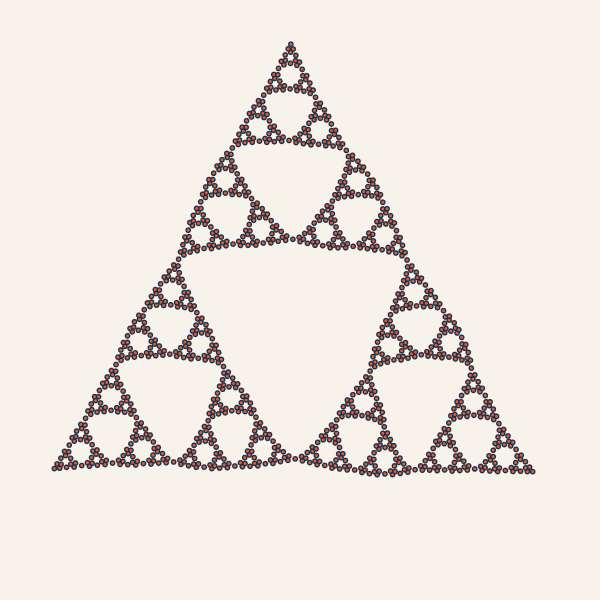
A completed Sierpinski triangle layout. Play the trace on the website to see vertices introduced and refined.

Reproduce this showcase · Get started · Choose a task · Explore the gallery

Its primary unweighted and weighted workflows target 2D and 3D, while opt-in weighted-GRIP, metric-MDS, and edge-KK workflows also support higher-dimensional embeddings. The main workflow is:

grip(metric = "hop") for topology-first layouts,
grip(metric = "edge_length") when edge lengths define the graph metric,
compare.layouts() and score.layout() for real-data layout selection,
trace.grip() with the same metric choice for diagnostics.

The package also includes advanced public experimental geodesic-KK utilities for weighted-layout scoring and polish. It builds on the GRIP (Graph dRawing with Intelligent Placement) method described in Gajer & Kobourov (2002) and Gajer, Goodrich & Kobourov (2004).

Installation

Released package

install.packages("grip")

The CRAN package page provides the manual and vignettes for the released version. CRAN currently provides 0.2.0, with four guides. Its metric.mds() performs classical scaling. This README and the package website describe development version 0.2.0.9001, which adds the function and synthetic-family guides and changes metric.mds() to raw-stress minimization. Use packageVersion("grip") to check your installation and read the MDS migration guide when moving to the development version.

Development package

Installing from source requires R and a C++17 toolchain (Rtools on Windows or command-line developer tools on macOS). For the package plus offline guides, also install Pandoc and the vignette-building R packages:

install.packages(c("remotes", "knitr", "rmarkdown"))
remotes::install_github("pgajer/grip", build_vignettes = TRUE)

For a smaller installation, omit vignette building and use the rendered website guides:

remotes::install_github("pgajer/grip", build_vignettes = FALSE)

Vignette building is off by default in remotes. The no-build route does not include the six offline guides. Optional viewers and numerical backends are needed only for workflows that use them; for example, install smacof to run the development metric.mds() method.

Quick start

This small mesh gives an immediate first result. It is a smaller example of graph drawing, not the level-6 construction shown above.

library(grip)
edges <- edges.mesh(4, 5)
coords <- grip(edges, n = 20, dim = 2, preset = "mesh", seed = 11)
plot.layout(coords, edges = edges, pch = 16, cex = 0.7,
            main = "A 4 by 5 mesh")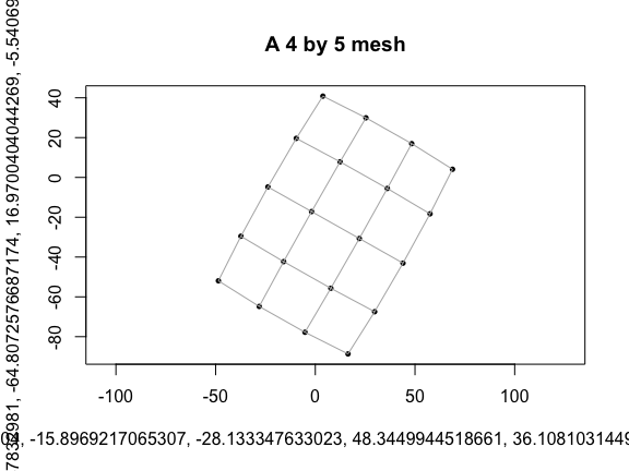

A 4 by 5 mesh drawn with the mesh preset; rows and columns remain visible.

quality <- score.layout(coords, edges = edges, n = 20,
                        sample.size.stress = 200, stress.seed = 11,
                        edge.crossings = "never")
quality[, c("sampled.stress", "edge.length.cv")]
#>   sampled.stress edge.length.cv
#> 1      0.1376255     0.06182833

Sampled stress compares drawn separation with graph hop distances after fitting a common scale; zero means exact agreement on the sampled pairs. The edge-length coefficient of variation measures relative variation in drawn edge lengths, useful here because the mesh is unweighted. Neither number certifies recovery of a reference shape. Try dim = 3 with plot.layout(coords, edges = edges, projection = "ortho") for a static 3D view.

From R, start with help("grip-package", package = "grip") or vignette("grip-examples", package = "grip") when installed guides are available. The function guide explains graph conventions, score meanings, and the next workflow.

Features

Multiscale force-directed layout in 2D and 3D via C++ (Rcpp).
A unified grip() interface for hop-metric and edge-length-metric layouts.
Opt-in multiscale weighted layout in dimensions greater than 3 via weighted.grip.nd(), with higher-dimensional metric-MDS and edge-KK workflows available through classical.mds(), metric.mds(), and edge.kk(). classical.mds() uses classical scaling; metric.mds() minimizes raw distance stress through the optional smacof package. In versions through 0.2.0, metric.mds() performed classical scaling: use classical.mds() to preserve that behavior. Edge-KK defaults to init = "classical_mds"; explicit init = "metric_mds" now requests stress minimization.
Layout comparison and quality scoring across seeds and parameter settings (compare.layouts(), score.layout()).
Multiscale trace diagnostics for both metrics via trace.grip().
Advanced public experimental geodesic-KK utilities for weighted-layout scoring and polish (prepare.geodesic.kk(), score.geodesic.kk(), prepare.landmark.geodesic.kk(), score.landmark.geodesic.kk()).
Synthetic graph-family helpers for benchmark and geometry-rich examples.
Handles disconnected graphs automatically (component packing).
Tuned presets for common graph families (see table below).
Static 3D projection for vignettes and reports (plot.layout(projection = "ortho"), project.3d()).

Presets

Family	Preset	Tuned on
Rectangular grid or lattice	`preset = "mesh"`	`8x8` and `12x12` meshes
Sierpinski carpet	`preset = "carpet"`	Level 3 and 4 carpets
Tree-like graph	`preset = "tree"`	Binary trees, depths 5 and 6
3D torus or cylinder	`preset = "torus"`	Torus sizes `8x8` through `20x20`

Presets set sensible defaults for the GRIP parameters. Any explicit argument you pass overrides the preset value.

Choosing a workflow

Start with grip(metric = "hop"), the default, when topology should define the multiscale hierarchy and graph neighborhoods.
Use grip(metric = "edge_length") when positive edge lengths should also define shortest-path distances, hierarchy construction, neighborhoods, and insertion anchors.
Use compare.layouts() and score.layout() when the graph is important enough to justify a candidate shortlist rather than a single run.
Use trace.grip() with the corresponding metric when you need to diagnose how a solve evolved.
Add GKK/LGKK only after you already have weighted candidate layouts and need geodesic-aware scoring or polish; these are advanced public experimental tools rather than the default starting point.

The historical argument names edge_weights and weight_list represent positive edge lengths, not connection strengths. With metric = "hop", supplied lengths set adjacent-edge force targets while standard GRIP hierarchy and neighborhood searches still count hops. With metric = "edge_length", the lengths also define weighted shortest paths throughout the multiscale engine and are median-normalized by default. See ?grip for the complete semantics and normalization options.

Gallery

The showcase recipes provide construction traces for the triangle and carpet, plus synchronized saddle rotations. The website uses still previews with explicit playback controls; the README links to those controls. The Sierpinski traces show algorithm steps. The saddle displays rotate saved coordinates, not solver iterations; their frozen fitting provenance is described alongside the recipe.

Graph-path fidelity, straight-line separation, and agreement with reference coordinates measure different aspects of a drawing. See Choose a score before interpreting a visual comparison.

More examples

Edge-list input (2D, circle placement)

edges <- edges.cycle(18)
coords <- grip(edges, n = 18, dim = 2, placement = "circle", seed = 2)
plot.layout(coords, edges, pch = 16, cex = 0.7)

Edge-length-metric adjacency list (geometry-aware)

adj_list <- list(c(2), c(1, 3), c(2, 4), c(3))
weight_list <- list(c(1.0), c(1.0, 2.0), c(2.0, 1.5), c(1.5))
coords <- grip(
  adj_list = adj_list, weight_list = weight_list,
  metric = "edge_length", n = 4, dim = 2, seed = 12
)
plot.layout(coords)

3D layout with static projection

edges <- edges.torus(8, 12)
coords <- grip(edges, n = max(edges), dim = 3, preset = "torus", seed = 3)
plot.layout(coords, edges, projection = "ortho", main = "Torus (8x12)")

Layout comparison

For real-world graphs without a known target layout, compare.layouts() compares candidates across seeds and reports quality metrics. Use params.from.summary() to extract the winning parameters for reuse.

edges <- edges.mesh(10, 10)
cmp <- compare.layouts(edges, n = 100, dim = 2,
                            candidates = c("default", "mesh"),
                            seeds = 1:3)
cmp$summary[, c("candidate", "score.composite", "sampled.stress.mean")]

Documentation

A development installation built with vignettes contains six guides, listed by vignette(package = "grip"):

Finding your way around grip — a task-oriented function catalog, metric and score choices, and detailed help. Open with vignette("function-guide", package = "grip").
Synthetic graph families and layout examples — reproducible graph bundles, static drawings, and reference-coordinate comparisons. Open with vignette("synthetic-graph-families", package = "grip").
Getting Started with grip — the shortest path through the default unweighted workflow, with guidance on when to switch to weighted, trace, or comparison workflows.
Weighted Graph Layouts with grip — geometry-aware layouts, geodesic scoring, and 2D-versus-3D decisions for weighted graphs.
Choosing Layouts for Real Data — a step-by-step workflow using the Zachary karate club and Krackhardt kite examples, plus a larger weighted HMP/U01 case study.
Tracing and Diagnosing Layouts — frame-by-frame tracing for understanding how a solve evolves.

The pkgdown site also includes companion articles such as the interactive explorer guide, the HMP/U01 object-structure note, the comparison article, and the synthetic-family gallery.

The geodesic-KK helpers are public and documented in the reference index, but they are intentionally positioned as advanced experimental tools layered on top of the main weighted workflow.

Citation

If you use grip in published work, please cite the underlying algorithm:

Gajer, P. and Kobourov, S.G. (2002). GRIP: Graph dRawing with Intelligent Placement. Journal of Graph Algorithms and Applications, 6(3), 203–224. doi: 10.7155/jgaa.00052

Gajer, P., Goodrich, M.T. and Kobourov, S.G. (2004). A multi-dimensional approach to force-directed layouts of large graphs. Computational Geometry, 29(1), 3–18. doi: 10.1016/j.comgeo.2004.03.014

License

GPL (>= 3)

Development

The developer map traces graph validation, preparation, engines, results, and displays, and lists source regeneration and full-dependency checks. The public workflow remains grip() → layout.coords() → plot.layout() / score.layout().