Synthetic graph families and layout examples • grip

Choose a synthetic family to make a layout question reproducible. A tree isolates branching and edge-length effects; a masked grid adds holes and bottlenecks; a surface bundle supplies reference coordinates. These examples use small graphs to demonstrate the workflow, not to rank layout methods. For the complete function catalog and score definitions, see Finding your way around grip.

Choose the kind of input you need

Need	Public entry points	Output
Topology alone	`edges.path()`, `edges.mesh()`, `edges.kary.tree()`, the other primitive `edges.*()` generators	Two-column edge matrix; no bundled reference coordinates or lengths.
A finite perforated grid	`keep.periodic.holes()`, `keep.asymmetric.notches()`, `keep.slit.channels()`, `keep.staggered.windows()`, then `occupied.mesh.surface.graph()`	A keep matrix followed by a complete weighted graph bundle.
A recursive pattern	Square `mask.()` helpers, cubic `mask.cube.()` arrays, or triangle/tetrahedron masks, then the matching `recursive.*.surface.graph()`	A mask followed by a recursively generated weighted bundle.
A regular reference surface	`mesh.surface.graph()`, `cylinder.surface.graph()`, `sphere.surface.graph()`, `torus.surface.graph()`	Edges, lengths, 3D reference coordinates, and parameters.
Irregular surfaces or volumes	The `irregular..surface.graph()` and `irregular..solid.graph()` families	Deterministic geometric constructions; “irregular” does not imply random sampling.
Triangular-lattice or polyhedral topology	The three `triangulated.*.surface.graph()` families	Graph edges and reference coordinates; the public bundles do not expose triangular faces.
Randomly sampled rectangle	`sampled.rectangle.surface.graph()` or plural `sampled.rectangle.surface.graphs()`	One graph or a sequence on a shared sampled point set.
Intrinsic lengths without an embedding	`kary.tree.weighted.graph()`	Tree edges, lengths, depths, parents, and edge metadata.

The website gallery illustrates more families. Use complete public bundles; standalone embeddings and specialized edge builders used inside them are internal functions. A name ending in surface.graph is not a promise of a triangle mesh: occupied-cube families, for example, connect occupied cells and can include interior vertices.

Read a bundle before using it

library(grip)
mesh <- mesh.surface.graph(3, 4, surface = "saddle", normalize = "none")
names(mesh)
#>  [1] "edges"          "n"              "edge_weights"   "coords_surface"
#>  [5] "coords_param"   "weight_scale"   "family"         "surface"       
#>  [9] "connectivity"   "normalize"      "label"
c(vertices = mesh$n, edges = nrow(mesh$edges),
  reference_dimensions = ncol(mesh$coords_surface))
#>             vertices                edges reference_dimensions 
#>                   12                   17                    3
head(mesh$edges)
#>      [,1] [,2]
#> [1,]    1    5
#> [2,]    1    2
#> [3,]    2    6
#> [4,]    2    3
#> [5,]    3    7
#> [6,]    3    4

Field	Meaning and ordering
`edges`	Integer matrix with two columns, one undirected edge per row; endpoints are 1-based vertex indices.
`n`	Total number of vertices. Use this instead of `max(edges)` so isolated vertices are retained.
`edge_weights`	Positive lengths parallel to edge rows. These are traversal lengths, not strengths.
`coords_surface`	When supplied, an `n` by 3 reference-coordinate matrix. Row `i` is vertex `i`, in the same order as the edge endpoints. Tree bundles omit it.
`coords_param`	When supplied, coordinates before the geometric deformation. Often `n` by 2, but polyhedra and volumetric families can use three columns. These are not automatically layout targets.
`weight_scale`	Divisor used to normalize raw lengths: supplied length equals raw length divided by `weight_scale`. The reference coordinates remain in their original units.
`normalize`, `family`, `label`, and construction controls	Record the selected normalization and family-specific settings. Exact fields differ by constructor.

Most geometric families induce lengths from the Euclidean distances between reference endpoints. kary.tree.weighted.graph() assigns lengths intrinsically. Sampled rectangles also return raw_edge_weights (3D endpoint distances) and iknn_witness_edge_weights (intersection-neighbor construction diagnostics). Even with graph_space = "param", the final sampled-rectangle lengths use 3D endpoint distances; graph_space changes graph construction.

Do not assume a shared schema beyond the documented constructor fields. The plural sampled-rectangle function returns a container with $graphs, $k, $k_statistics, and shared coordinate matrices; pass one member of $graphs to the layout workflow. It sorts and deduplicates the supplied neighborhood sizes. No public bundle used here supplies faces or triangles. score.surface() needs explicit triangle connectivity supplied separately; it cannot infer a surface from these edge lists.

Ordering is part of reproducibility. The rectangular mesh enumerates each row from left to right. Mask matrices use display orientation (top row first, left column first); occupied-cell coordinates and graph indices share that order. Sphere bundles put the north pole first, then latitude rings from north to south, then the south pole. Trees put the root first and enumerate children by parent and child slot. For other families, retain the constructor’s returned order rather than reconstructing it from a drawing. Reordering rows requires remapping edges and every reference and metadata field together.

Example 1: a tree with intrinsic edge lengths

Use a primitive path when you need only topology:

path.edges <- edges.path(7)
path.coords <- grip(path.edges, n = 7, dim = 2, preset = "tree", seed = 21)
stopifnot(identical(dim(path.edges), c(6L, 2L)))

A complete weighted tree separates depth-dependent tapering from child-slot asymmetry. Here a binary tree has three levels below the root (15 vertices). It has no generating reference coordinates; a graph-distance diagnostic is therefore the appropriate first score.

tree <- kary.tree.weighted.graph(
  k = 2, depth = 3, depth_decay = 0.8,
  branch_spread = 0.25, normalize = "none"
)
knitr::kable(head(tree$edge_table), digits = 3)

parent	child	parent_depth	child_depth	branch_index	raw_weight	edge_weight
1	2	0	1	1	0.875	0.875
1	3	0	1	2	1.125	1.125
2	4	1	2	1	0.700	0.700
2	5	1	2	2	0.900	0.900
3	6	1	2	1	0.700	0.700
3	7	1	2	2	0.900	0.900

tree.coords <- grip(tree$edges, n = tree$n,
                    edge_weights = tree$edge_weights,
                    metric = "edge_length", length_normalization = "none",
                    dim = 2, preset = "tree", seed = 21)
plot.layout(tree.coords, edges = tree$edges,
            vertex.col = tree$vertex_depth + 1L, pch = 16,
            main = "Intrinsic lengths on a binary tree")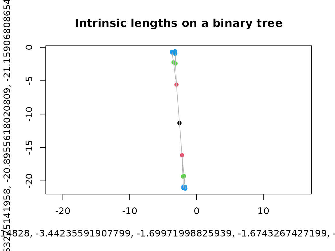

A branching tree drawn using intrinsic positive edge lengths; its connectivity and edge-length variation are visible.

tree.score <- score.layout(tree.coords, edges = tree$edges, n = tree$n,
                            edge_weights = tree$edge_weights,
                            sample.size.stress = 150, stress.seed = 21,
                            edge.crossings = "never")
knitr::kable(tree.score[, c("sampled.stress", "edge.length.cv")], digits = 3)

sampled.stress	edge.length.cv
0.346	0.522

parent has one entry per vertex and uses 0 for the root’s missing parent; vertex_depth starts at 0. edge_table follows the edge rows and records parent, child, both depths, child slot, raw length, and normalized length. Unequal drawn edges are intentional here, so a low edge-length coefficient of variation is not the goal. Weighted sampled stress evaluates chords against tree-path distances after fitting scale. Branching tree metrics cannot in general be preserved exactly as Euclidean separations in two dimensions.

Example 2: a recursive graph with holes

A keep mask describes which cells survive each subdivision. The border of a 3 by 3 mask removes the center at each step. At level 2 there are 64 retained cells. This example uses a flat lift (amplitude = 0) and omits lengths when fitting and scoring, so both operations use hop counts.

keep <- mask.border(3)
keep
#>      [,1]  [,2] [,3]
#> [1,] TRUE  TRUE TRUE
#> [2,] TRUE FALSE TRUE
#> [3,] TRUE  TRUE TRUE
carpet <- recursive.mask.grid.surface.graph(
  mask = keep, level = 2, surface = "saddle", amplitude = 0
)
stopifnot(carpet$n == 64L, nrow(carpet$coords_param) == carpet$n)
carpet.coords <- grip(carpet$edges, n = carpet$n,
                      metric = "hop", dim = 2, preset = "carpet", seed = 22)

op <- par(mfrow = c(1, 2), mar = c(3, 3, 2, 1))
plot.layout(carpet$coords_param, edges = carpet$edges, pch = 16, cex = 0.5,
            main = "Generating grid")
plot.layout(carpet.coords, edges = carpet$edges, pch = 16, cex = 0.5,
            main = "Hop-metric drawing")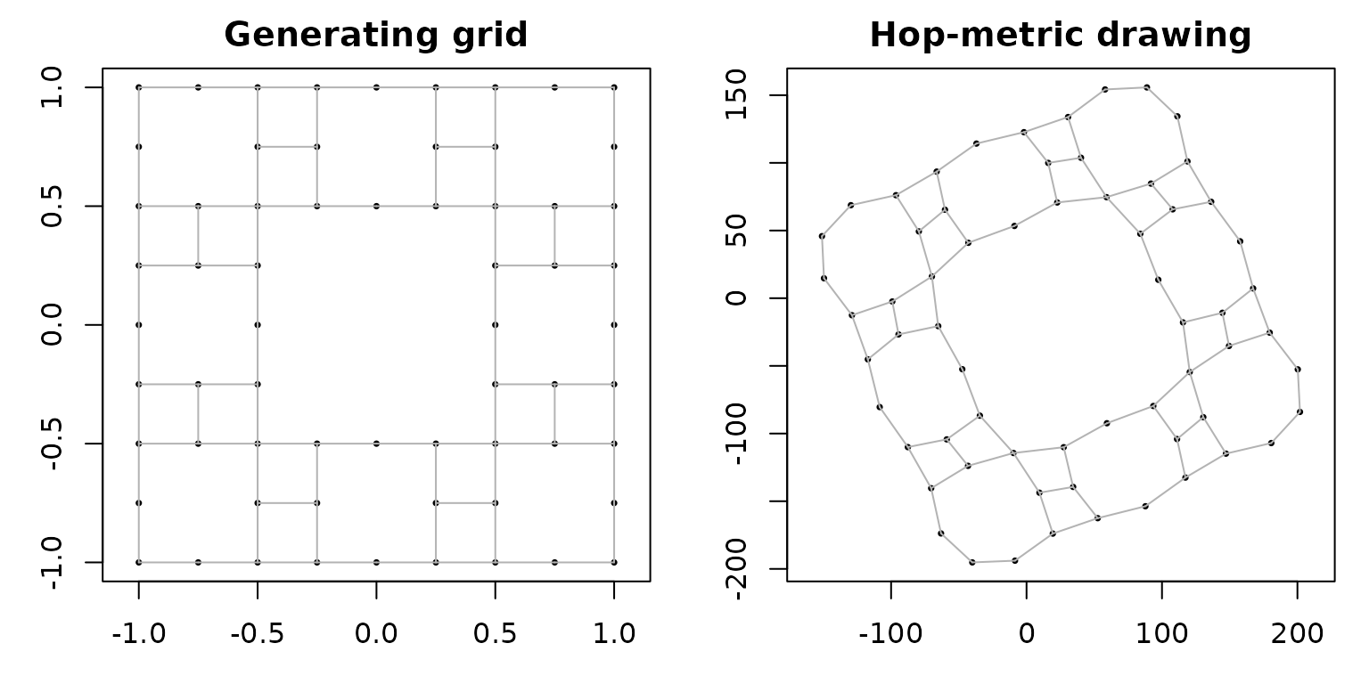

Reference grid and GRIP drawing of a recursive carpet with holes, shown side by side.

par(op)

carpet.score <- score.layout(carpet.coords, edges = carpet$edges, n = carpet$n,
                              sample.size.stress = 300, stress.seed = 22,
                              edge.crossings = "never")
carpet.score$sampled.stress
#> [1] 0.1061113

The layout preserves the graph’s vertex and edge identities, but it need not reproduce the original square arrangement. Holes and narrow connections make this a useful example for tracing. A different keep pattern can disconnect a graph or isolate cells; grip() packs components by default. Such packing is not evidence of distances between disconnected components.

Square and cubic recursive grids require level >= 1. Triangle and tetrahedron recursions and triangulated polyhedra also allow level 0. Triangle masks have four named child slots; tetrahedron masks have four corner slots. A cubic keep array is not interchangeable with either. Increasing depth multiplies the retained cells, so inspect n before launching a layout or all-pairs score.

Example 3: graph fidelity versus reference recovery

An octahedron subdivided once gives 18 vertices and a three-dimensional reference configuration. The two fits below keep topology, vertex order, supplied lengths, seed, dimension, preset, and iteration controls fixed. Both receive the same unnormalized lengths. Hop mode uses those lengths for adjacent-edge forces; edge-length mode additionally uses them for graph neighborhoods and hierarchy construction. Its solver normalization is set to "none" to retain the same input length scale.

surface <- triangulated.polyhedron.surface.graph(
  base = "octahedron", level = 1, surface = "inflated", normalize = "none"
)
common <- list(edges = surface$edges, n = surface$n,
               edge_weights = surface$edge_weights, dim = 3,
               preset = "mesh", rounds = 40, final_rounds = 60, seed = 23)
fits <- list(
  hop = do.call(grip, c(common, list(metric = "hop"))),
  edge_length = do.call(grip, c(common, list(
    metric = "edge_length", length_normalization = "none")))
)
stopifnot(surface$n == 18L,
          all(vapply(fits, function(x) all(is.finite(x)), logical(1))))
reference.scores <- lapply(fits, score.coordinates,
                           reference = surface$coords_surface,
                           alignment = "similarity")
summary <- do.call(rbind, lapply(names(fits), function(method) {
  graph.score <- score.layout(
    fits[[method]], edges = surface$edges, n = surface$n,
    edge_weights = surface$edge_weights, sample.size.stress = 200,
    stress.seed = 23, edge.crossings = "never"
  )
  data.frame(method = method,
             weighted_chord_stress = graph.score$sampled.stress,
             reference_relative_rmse = reference.scores[[method]]$relative_rmse,
             alignment_scale = reference.scores[[method]]$scale)
}))
knitr::kable(summary, digits = 3)

method	weighted_chord_stress	reference_relative_rmse	alignment_scale
hop	0.124	0.01	0.039
edge_length	0.124	0.01	0.039

Both drawings are scored against the same weighted graph distances, with the same pair sampling settings. The coordinate score separately uses the same reference and vertex correspondence, fitting translation, an orthogonal transformation (including reflection), and uniform scale. Relative coordinate RMSE is root mean squared vertex displacement divided by the reference’s RMS radius. Similarity alignment removes overall size differences, so it does not establish recovery of absolute length scale. Use alignment = "rigid" when scale must count as error.

op <- par(mfrow = c(1, 3), mar = c(1, 1, 2, 1))
plot.layout(surface$coords_surface, edges = surface$edges,
            projection = "ortho", main = "Reference")
for (method in names(fits)) {
  plot.layout(reference.scores[[method]]$coords, edges = surface$edges,
              projection = "ortho",
              main = if (method == "hop") "Hop metric" else "Edge-length metric",
              vertex.col = "#215A87")
}

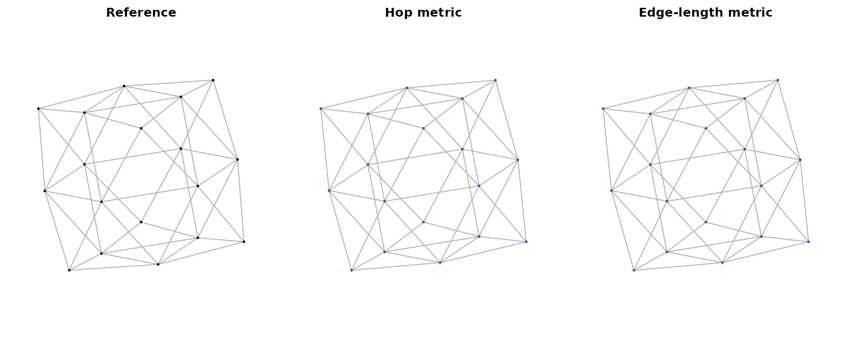
Static projections of the reference surface and the hop- and edge-length-metric layouts, aligned for comparison.

par(op)

These are static orthographic views of 3D coordinates, not new 2D fits. Scores above use all three columns. The generating coordinates provide one reference: graph symmetries, bending, missing constraints, and the choice of objective can permit other drawings. Matching graph-path distances, matching endpoint separations, and recovering this reference are distinct goals. Here the rounded scores agree closely, showing that the two metric choices can give similar results on a symmetric graph. One graph and one seed do not establish general superiority of either mode.

Reproducibility and practical limits

Primitive generators and the regular, recursive, and irregular families are deterministic for fixed construction arguments. The sampled-rectangle family uses random sampling: a supplied integer seed fixes that sample and restores the caller’s R random-number state; seed = NULL uses and advances the current stream. A plural call samples once for all requested neighborhood sizes. Graph sampling and layout fitting have separate seeds.

sample.one <- sampled.rectangle.surface.graph(n = 20, k = 4, seed = 24)
sample.two <- sampled.rectangle.surface.graph(n = 20, k = 4, seed = 24)
stopifnot(identical(sample.one$edges, sample.two$edges),
          identical(sample.one$coords_surface, sample.two$coords_surface))
c(vertices = sample.one$n, edges = nrow(sample.one$edges))
#> vertices    edges 
#>       20       54

For grip(), pass an explicit seed (the default is 6); NULL uses the current time rather than the caller’s R random stream. Record the package version, graph arguments, vertex order, graph and solver normalization, layout controls, and scoring seeds. Fixed seeds aid repeatability within an implementation; they are not promises of identical floating-point results across future versions and platforms.

The surface and solid bundles here return three reference columns, while grip() fits either 2D or 3D. Higher-dimensional layout workflows are described in the function guide; changing layout dimension does not create a higher-dimensional reference bundle. Sphere and wrapped families have minimum grid-size restrictions; intrinsic trees can have depth 0, with one vertex and no edges. Use constructor help for parameter bounds.

No example here needs Shiny, rgl, an interactive device, or a browser. For larger families, first inspect the graph size and use modest sampled scores; full shortest-path matrices and route caches can dominate memory. Optional interactive exploration and the gallery are website follow-ups. The installed weighted-layout guide and real-data guide develop the corresponding workflows.