
Two real-data workflows
For real graphs there is usually no single correct picture waiting to be recovered. The practical goal is to find a layout that is:
- faithful to graph structure,
- visually coherent,
- and stable enough to trust.
In grip, that usually leads to one of two workflows:
- a combinatorial workflow for unweighted or
topology-first graphs, based on
compare.layouts()andscore.layout(), - a weighted workflow for graphs whose edge lengths
carry real geometry, based on
grip(metric = "edge_length"), weighted scoring, and often 3D layouts.
This vignette shows both patterns. The bundled karate-club and Krackhardt-kite graphs illustrate the first one. The bundled coarsened HMP/U01 graph illustrates the second.
The same package-level decision rule still applies:
- ordinary unweighted or topology-first graphs: start with
grip(),compare.layouts(), andscore.layout(), - weighted graphs with meaningful edge lengths: start with
grip(metric = "edge_length"), usually with 3D in the candidate set, - when a promising solve needs explanation rather than another run: add trace,
- when a smaller weighted candidate set needs stronger metric-aware comparison: add GKK/LGKK as advanced public experimental tools.
The small helpers below keep the plotting code compact.
read.extdata.csv <- function(file.name) {
  candidates <- c(
    system.file("extdata", file.name, package = "grip"),
    file.path("inst", "extdata", file.name),
    file.path("..", "inst", "extdata", file.name)
  )
  path <- candidates[file.exists(candidates)][1L]
  if (!length(path) || is.na(path) || !nzchar(path)) {
    stop("could not locate ", file.name)
  }
  utils::read.csv(path, stringsAsFactors = FALSE)
}

read.edge.csv <- function(file.name) {
  as.matrix(read.extdata.csv(file.name))
}

read.karate.club <- function() {
  labels <- read.extdata.csv("karate-club-membership.csv")
  labels <- labels[order(labels$vertex), , drop = FALSE]
  labels$club
}

compact.summary <- function(x) {
  keep <- intersect(c(
    "candidate",
    "preset",
    "rounds",
    "final.rounds",
    "num.nbrs",
    "repulsion.factor",
    "sampled.stress.mean",
    "edge.length.cv.mean",
    "sampled.nonedge.sep.ratio.mean",
    "cluster.separation.mean",
    "stability.procrustes.mean",
    "score.composite"
  ), names(x))
  x[, keep, drop = FALSE]
}

plot.layout.triptych <- function(layouts,
                                 edges,
                                 titles,
                                 vertex.cols = NULL) {
  if (is.null(vertex.cols)) {
    vertex.cols <- rep(list("black"), length(layouts))
  }
  op <- par(mfrow = c(1, length(layouts)), mar = c(1.2, 1.2, 3.2, 1.2))
  on.exit(par(op), add = TRUE)
  for (i in seq_along(layouts)) {
    plot.layout(
      layouts[[i]],
      edges,
      projection = if (ncol(layouts[[i]]) == 3L) "ortho" else NULL,
      vertex.col = vertex.cols[[i]],
      edge.col = "gray82",
      main = titles[[i]]
    )
  }
}

edge.matrix.from.adj <- function(adj.list) {
  edges <- list()
  idx <- 0L
  for (u in seq_along(adj.list)) {
    nbrs <- adj.list[[u]]
    nbrs <- nbrs[nbrs > u]
    if (!length(nbrs)) next
    for (v in nbrs) {
      idx <- idx + 1L
      edges[[idx]] <- c(u, v)
    }
  }
  do.call(rbind, edges)
}

read.hmp.vignette.results <- function() {
  path <- system.file(
    "extdata", "hmp_u01_gc_coarse", "vignette_results.rds",
    package = "grip"
  )
  if (!nzchar(path)) {
    stop("could not locate bundled HMP/U01 vignette results")
  }
  readRDS(path)
}
Workflow 1: shortlist candidates on an unweighted real graph
The karate-club network is a good real-data starting point because it
is small, interpretable, and comes with a known split between the
Mr. Hi and Officer factions (Zachary 1977).
karate.edges <- read.edge.csv("karate-club-edges.csv")
karate.n <- max(karate.edges)
karate.club <- read.karate.club()
karate.cols <- ifelse(karate.club == "Mr. Hi", "#1b9e77", "#d95f02")

karate.cmp <- compare.layouts(
  edges = karate.edges,
  n = karate.n,
  dim = 3,
  candidates = c("default", "tree", "mesh"),
  clusters = karate.club,
  seeds = 1:3,
  sample.size.stress = 1000L,
  sample.size.nonedge = 2000L,
  edge.crossings = "never",
  return.layouts = TRUE
)

knitr::kable(compact.summary(karate.cmp$summary), digits = 3)| candidate | preset | rounds | final.rounds | num.nbrs | repulsion.factor | sampled.stress.mean | edge.length.cv.mean | sampled.nonedge.sep.ratio.mean | cluster.separation.mean | stability.procrustes.mean | score.composite |
|---|---|---|---|---|---|---|---|---|---|---|---|
| default | NA | 20 | 25 | 10 | 1.0 | 0.323 | 0.207 | 0.206 | 1.134 | 0.427 | 0.395 |
| mesh | mesh | 128 | 128 | 20 | 1.5 | 0.187 | 0.225 | 0.000 | 2.049 | 0.202 | 0.421 |
| tree | tree | 64 | 160 | 8 | 0.0 | 0.347 | 0.524 | 0.012 | 3.965 | 0.075 | 0.684 |
plot.layout.triptych(
  layouts = list(
    karate.cmp$layouts$default[["1"]],
    karate.cmp$layouts$tree[["1"]],
    karate.cmp$layouts$mesh[["1"]]
  ),
  edges = karate.edges,
  titles = c("default", "tree", "mesh"),
  vertex.cols = rep(list(karate.cols), 3)
)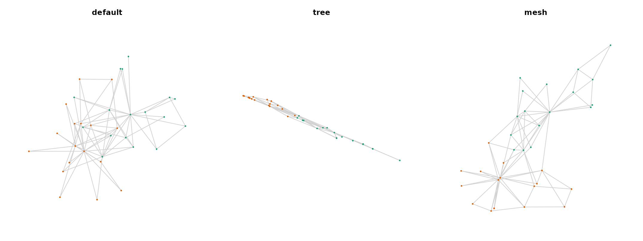
This is the main combinatorial real-data pattern:
- compare a small number of plausible candidates,
- use several seeds,
- read the score table before picking a favorite picture,
- and use metadata-aware metrics such as
cluster.separationwhen they are genuinely meaningful.
A small local search around the strongest region
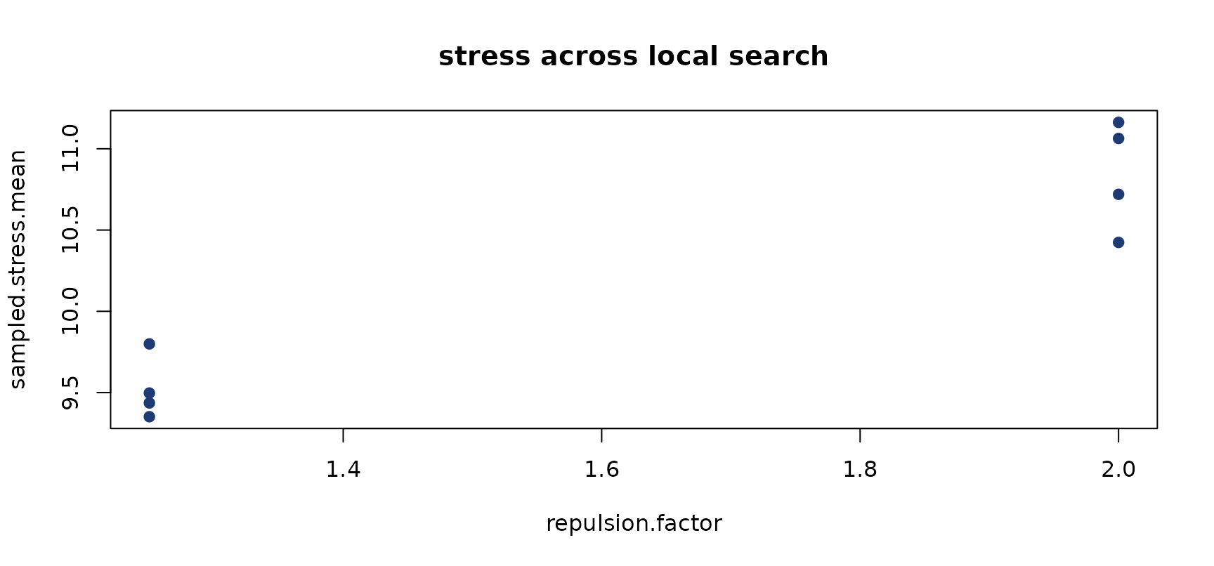
After the first shortlist, it is usually better to search locally than to launch a wide, blind parameter sweep.
karate.search <- compare.layouts(
  edges = karate.edges,
  n = karate.n,
  dim = 3,
  search = list(
    candidate.prefix = "karate.search",
    preset = c("tree"),
    rounds = c(96L, 128L),
    final_rounds = c(192L, 224L),
    repulsion_factor = c(1.25, 2.0)
  ),
  clusters = karate.club,
  seeds = 1:3,
  sample.size.stress = 1000L,
  sample.size.nonedge = 2000L,
  edge.crossings = "never",
  return.layouts = TRUE
)

knitr::kable(head(compact.summary(karate.search$summary), 6), digits = 3)| candidate | preset | rounds | final.rounds | num.nbrs | repulsion.factor | sampled.stress.mean | edge.length.cv.mean | sampled.nonedge.sep.ratio.mean | cluster.separation.mean | stability.procrustes.mean | score.composite |
|---|---|---|---|---|---|---|---|---|---|---|---|
| karate.search.rounds.128.final_rounds.192.repulsion_factor.125 | tree | 128 | 192 | 8 | 1.25 | 0.232 | 0.196 | 0 | 1.801 | 0.285 | 0.353 |
| karate.search.rounds.128.final_rounds.224.repulsion_factor.125 | tree | 128 | 224 | 8 | 1.25 | 0.237 | 0.193 | 0 | 1.793 | 0.276 | 0.353 |
| karate.search.rounds.96.final_rounds.192.repulsion_factor.2 | tree | 96 | 192 | 8 | 2.00 | 0.229 | 0.199 | 0 | 1.819 | 0.337 | 0.376 |
| karate.search.rounds.96.final_rounds.192.repulsion_factor.125 | tree | 96 | 192 | 8 | 1.25 | 0.237 | 0.189 | 0 | 1.733 | 0.301 | 0.429 |
| karate.search.rounds.96.final_rounds.224.repulsion_factor.2 | tree | 96 | 224 | 8 | 2.00 | 0.238 | 0.195 | 0 | 1.760 | 0.338 | 0.526 |
| karate.search.rounds.128.final_rounds.192.repulsion_factor.2 | tree | 128 | 192 | 8 | 2.00 | 0.243 | 0.196 | 0 | 1.776 | 0.300 | 0.541 |
op <- par(mfrow = c(1, 2), mar = c(4, 4, 2.2, 1))
on.exit(par(op), add = TRUE)

plot(
  karate.search$summary$repulsion.factor,
  karate.search$summary$sampled.stress.mean,
  pch = 19,
  col = "#1F3B73",
  xlab = "repulsion.factor",
  ylab = "sampled.stress.mean",
  main = "stress across local search"
)
plot(
  karate.search$summary$repulsion.factor,
  karate.search$summary$cluster.separation.mean,
  pch = 19,
  col = "#B24745",
  xlab = "repulsion.factor",
  ylab = "cluster.separation.mean",
  main = "cluster separation across search"
)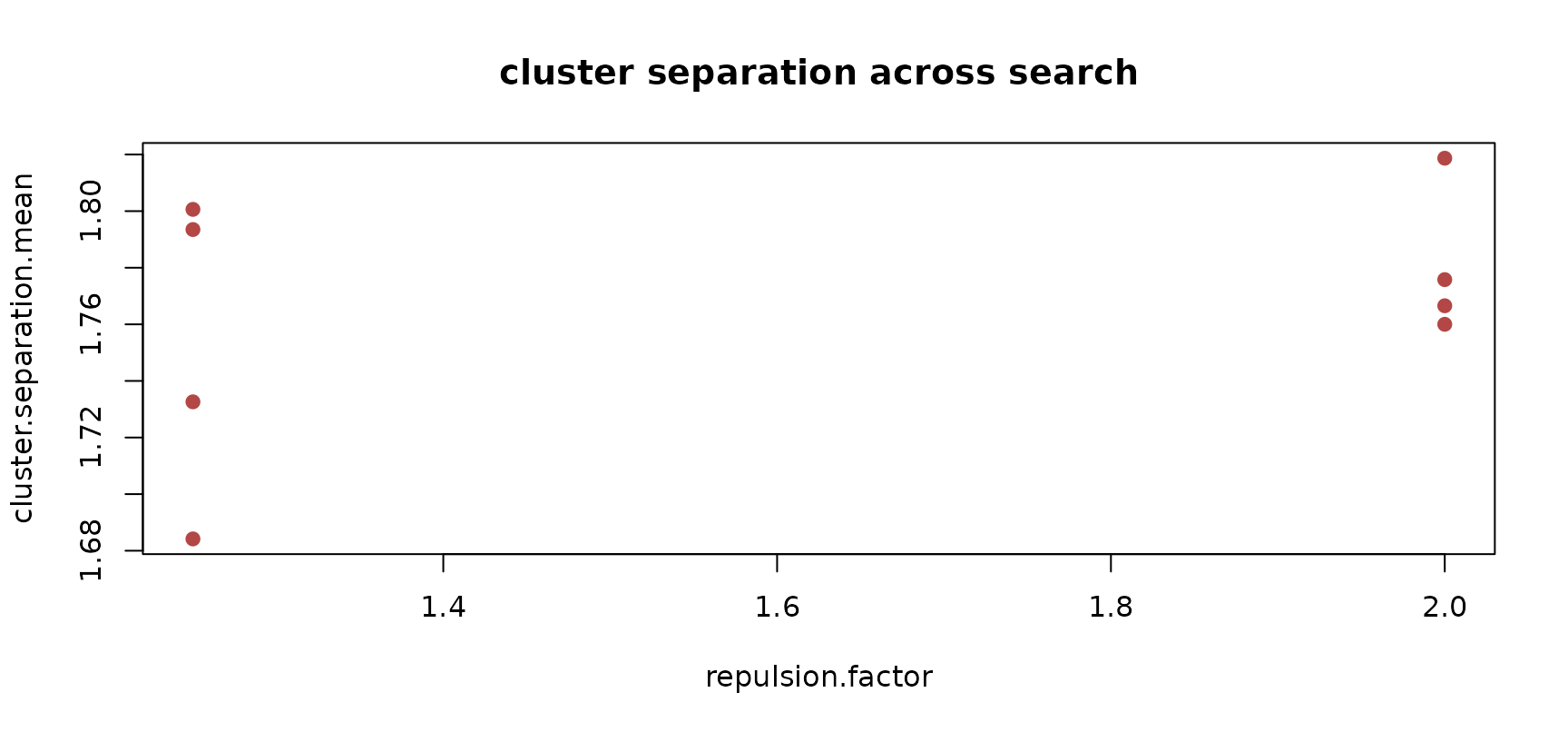
The point is not to overfit the graph. It is to identify a stable, sensible region of the parameter space.
A second small graph: direct scoring
Not every real-data task needs a comparison grid. On very small graphs it is often enough to realize one or two layouts and score them directly.
kite.edges <- read.edge.csv("krackhardt-kite-edges.csv")
kite.n <- max(kite.edges)

kite.coords <- grip(
  kite.edges,
  n = kite.n,
  dim = 2,
  preset = "tree",
  seed = 5
)

score.layout(kite.coords, edges = kite.edges, n = kite.n)
#>   n.vertices n.edges dim sampled.stress edge.length.cv median.edge.length
#> 1         10      18   2      0.3256882      0.7467341           1.131498
#>   sampled.nonedge.sep.ratio edge.crossings cluster.separation
#> 1                 0.3247241              2                 NA
plot.layout(
  kite.coords,
  kite.edges,
  main = "Krackhardt kite",
  pch = 16,
  cex = 0.9,
  edge.col = "gray80"
)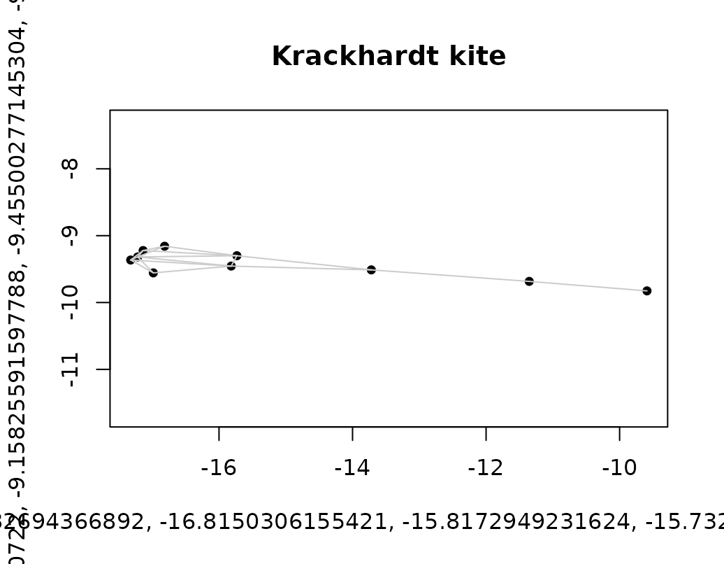
score.layout() is especially useful when:
- the layout was generated once and cached,
- the layout came from another tool,
- or you want to score a hand-curated final picture.
Workflow 2: when the real graph is weighted
Some real graphs are not just topological. Their edge lengths carry
information that should influence the layout itself. The bundled
hmp.u01.gc.coarse example is in that category: it is a
weighted, coarsened real-world graph from the HMP+U01 16S amplicon
analysis pipeline.
data(hmp.u01.gc.coarse)

hmp.graph.info <- data.frame(
  quantity = c(
    "coarse vertices",
    "weighted undirected edges",
    "selected k",
    "representation"
  ),
  value = c(
    hmp.u01.gc.coarse$graph_info$coarse_vertices,
    hmp.u01.gc.coarse$graph_info$edge_count,
    hmp.u01.gc.coarse$graph_info$selected_k,
    hmp.u01.gc.coarse$graph_info$representation
  ),
  stringsAsFactors = FALSE
)

hmp.weight.summary <- as.data.frame(t(summary(unlist(
  hmp.u01.gc.coarse$weight_list,
  use.names = FALSE
))))

knitr::kable(hmp.graph.info)| quantity | value |
|---|---|
| coarse vertices | 1828 |
| weighted undirected edges | 4656 |
| selected k | 3 |
| representation | >=1% relative abundance + PCA |
knitr::kable(hmp.weight.summary, digits = 4)| Var1 | Var2 | Freq |
|---|---|---|
| A | Min. | 0.0002 |
| A | 1st Qu. | 0.0409 |
| A | Median | 0.0990 |
| A | Mean | 0.1370 |
| A | 3rd Qu. | 0.1884 |
| A | Max. | 1.2078 |
A useful practical signal is that the edge-weight variation is large enough to matter.
hmp.weight.cv <- with(
  list(w = unlist(hmp.u01.gc.coarse$weight_list, use.names = FALSE)),
  stats::sd(w) / mean(w)
)

hmp.weight.cv
#> [1] 1.004854
For graphs like this, the weighted workflow differs from the combinatorial one:
- start with
grip(metric = "edge_length")rather thangrip(), - prefer 3D as the primary layout space,
- and assess geometry with a weighted graph-metric criterion when possible.
A plain grip() solve can still be useful here as a
topology-first baseline, but it should not be the default when the edge
lengths themselves matter scientifically.
The direct weighted-candidate pattern looks like this:
weighted.candidates <- list(
  weighted_default = grip(metric = "edge_length",
    adj_list = hmp.u01.gc.coarse$adj_list,
    weight_list = hmp.u01.gc.coarse$weight_list,
    n = length(hmp.u01.gc.coarse$adj_list),
    dim = 3,
    seed = 1
  ),
  weighted_irregular = grip(metric = "edge_length",
    adj_list = hmp.u01.gc.coarse$adj_list,
    weight_list = hmp.u01.gc.coarse$weight_list,
    n = length(hmp.u01.gc.coarse$adj_list),
    dim = 3,
    preset = "irregular",
    seed = 1
  )
)

weighted.scores <- lapply(weighted.candidates, function(coords) {
  score.layout(
    coords,
    adj_list = hmp.u01.gc.coarse$adj_list,
    weight_list = hmp.u01.gc.coarse$weight_list,
    n = length(hmp.u01.gc.coarse$adj_list),
    clusters = hmp.u01.gc.coarse$vertex_data$cst,
    sample.size.stress = 2000L,
    sample.size.nonedge = 5000L,
    edge.crossings = "never"
  )
})
For smaller weighted real graphs, it is also worth comparing candidate layouts with:
prepare.geodesic.kk()score.geodesic.kk()prepare.landmark.geodesic.kk()score.landmark.geodesic.kk()
because they assess retained-path length fidelity separately from sampled endpoint-distance stress. These score values are not interchangeable. These GKK/LGKK helpers are public, but they are best treated as advanced experimental tools layered on top of the main weighted workflow.
HMP/U01 as a large weighted case study
The package also ships a larger, more realistic weighted example:
hmp.u01.gc.coarse. This graph is large enough that a full
search is too heavy for a regular vignette build, so the package
includes bundled precomputed results for a representative 3D search.
hmp.results <- read.hmp.vignette.results()
hmp.edges <- edge.matrix.from.adj(hmp.u01.gc.coarse$adj_list)
hmp.cst <- hmp.u01.gc.coarse$vertex_data$cst
hmp.cst.levels <- sort(unique(hmp.cst))
hmp.cst.cols <- setNames(grDevices::hcl.colors(length(hmp.cst.levels), "Dark 3"),
                         hmp.cst.levels)
hmp.cst.col <- hmp.cst.cols[hmp.cst]

hmp.case.info <- data.frame(
  quantity = c(
    "source dataset",
    "representation",
    "selected k",
    "original giant-component vertices",
    "coarsened vertices",
    "weighted undirected edges"
  ),
  value = c(
    hmp.u01.gc.coarse$graph_info$source_dataset,
    hmp.u01.gc.coarse$graph_info$representation,
    hmp.u01.gc.coarse$graph_info$selected_k,
    hmp.u01.gc.coarse$graph_info$original_vertices,
    hmp.u01.gc.coarse$graph_info$coarse_vertices,
    hmp.u01.gc.coarse$graph_info$edge_count
  ),
  stringsAsFactors = FALSE
)

knitr::kable(hmp.case.info)| quantity | value |
|---|---|
| source dataset | HMP+U01 16S amplicon |
| representation | >=1% relative abundance + PCA |
| selected k | 3 |
| original giant-component vertices | 6474 |
| coarsened vertices | 1828 |
| weighted undirected edges | 4656 |
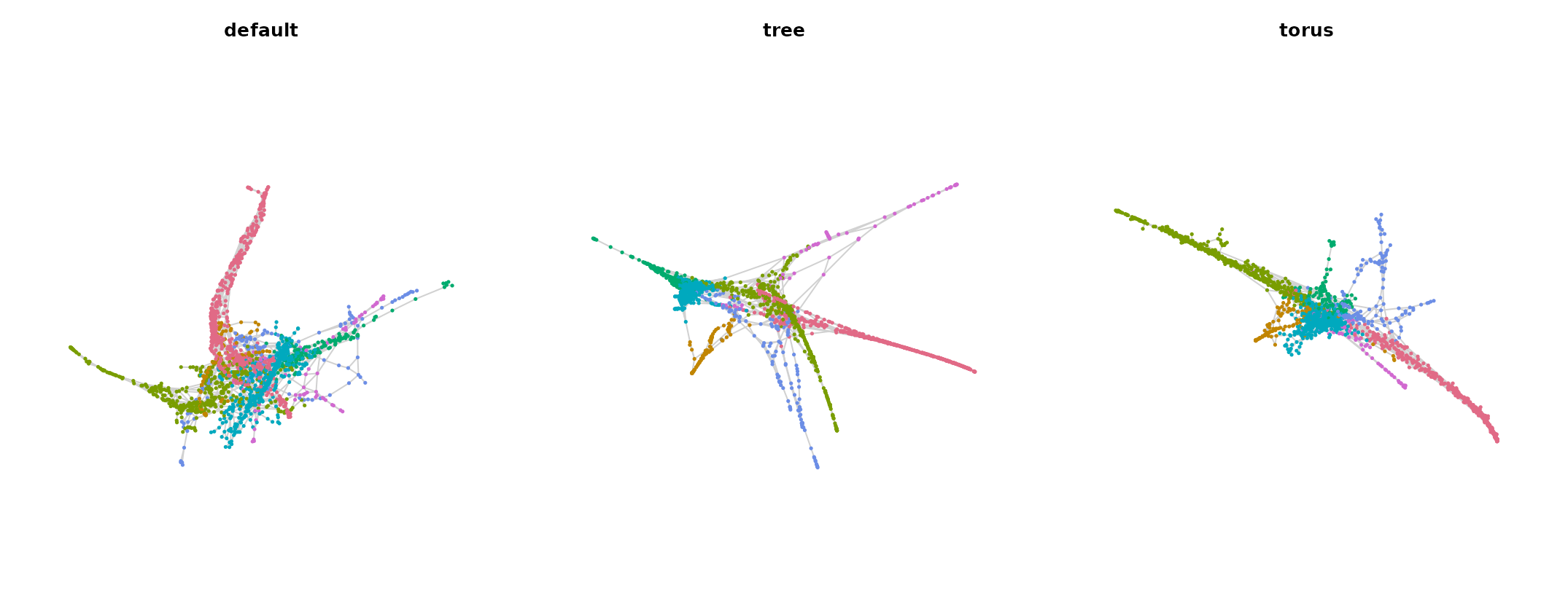
The bundled preset comparison used three 3D candidates:
defaulttreetorus
hmp.preset.keep <- c(
  "candidate",
  "sampled.stress.mean",
  "edge.length.cv.mean",
  "sampled.nonedge.sep.ratio.mean",
  "cluster.separation.mean",
  "score.composite"
)

knitr::kable(hmp.results$preset_summary[, hmp.preset.keep], digits = 3)| candidate | sampled.stress.mean | edge.length.cv.mean | sampled.nonedge.sep.ratio.mean | cluster.separation.mean | score.composite |
|---|---|---|---|---|---|
| default | 0.407 | 0.734 | 0.400 | 2.310 | 0.062 |
| torus | 0.461 | 0.962 | 0.115 | 3.401 | 0.625 |
| tree | 0.490 | 1.097 | 0.190 | 3.706 | 0.812 |
plot.layout.triptych(
  layouts = list(
    hmp.results$layouts$preset$default,
    hmp.results$layouts$preset$tree,
    hmp.results$layouts$preset$torus
  ),
  edges = hmp.edges,
  titles = c("default", "tree", "torus"),
  vertex.cols = rep(list(hmp.cst.col), 3)
)
For this graph, the useful next step was a small local search around the stronger region rather than a broad blind sweep.
hmp.local.keep <- c(
  "candidate",
  "rounds",
  "final.rounds",
  "repulsion.factor",
  "sampled.stress.mean",
  "cluster.separation.mean",
  "score.composite"
)

knitr::kable(
  head(hmp.results$local_search_summary[, hmp.local.keep], 4),
  digits = 3
)| candidate | rounds | final.rounds | repulsion.factor | sampled.stress.mean | cluster.separation.mean | score.composite |
|---|---|---|---|---|---|---|
| hmp.local.final_rounds.224.repulsion_factor.125 | 192 | 224 | 1.25 | 0.507 | 3.820 | 0.250 |
| hmp.local.final_rounds.288.repulsion_factor.125 | 192 | 288 | 1.25 | 0.506 | 3.763 | 0.312 |
| hmp.local.final_rounds.224.repulsion_factor.075 | 192 | 224 | 0.75 | 0.509 | 3.846 | 0.458 |
| hmp.local.final_rounds.288.repulsion_factor.075 | 192 | 288 | 0.75 | 0.510 | 3.785 | 0.979 |
top.local <- hmp.results$top_local_candidates
plot.layout.triptych(
  layouts = lapply(top.local, function(nm) hmp.results$layouts$local[[nm]]),
  edges = hmp.edges,
  titles = top.local,
  vertex.cols = rep(list(hmp.cst.col), length(top.local))
)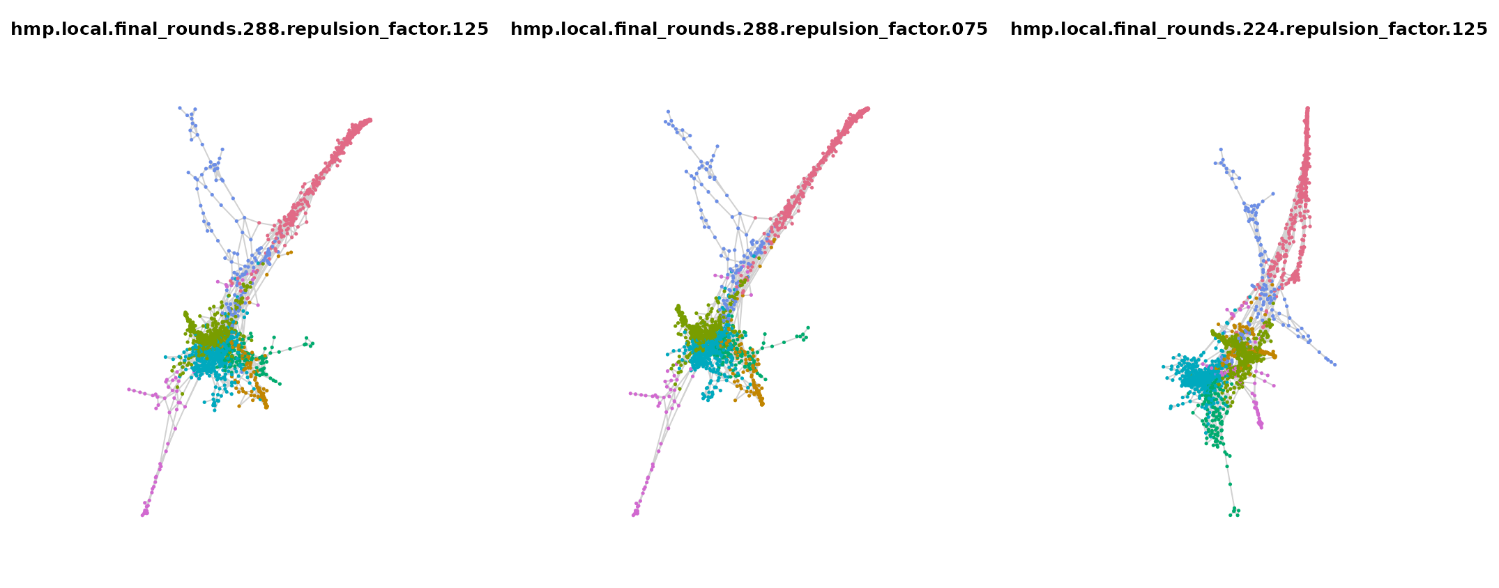
This is the large-graph weighted pattern in practice:
- keep the graph weighted,
- prefer 3D,
- use a short preset shortlist,
- then search locally around the strongest region,
- and interpret the final layouts together with domain labels such as CST.
For the HMP/U01-specific object structure, coarsening provenance, and
bundled artifact paths, see the companion article
HMP/U01 Weighted Graph Case Study.
Practical guidance
- Use
compare.layouts()for unweighted or topology-first real graphs. - Use a small candidate shortlist before any local search.
- Keep 3D in the candidate set when the graph is structurally rich.
- If edge lengths are scientifically meaningful, switch to
grip(metric = "edge_length"). - Use
trace.grip()ortrace.grip(metric = "edge_length")when a promising solve needs diagnosis rather than another broad sweep. - For weighted graphs, treat 3D as the primary evaluation space and use GKK/LGKK scoring only when the graph is small enough for those advanced experimental checks to be practical.
Related guides
For an API map, see Finding your way around grip. For reproducible bundles and reference scoring, see Synthetic graph families and layout examples. Both are installed vignettes; the broader gallery and interactive explorer are website-only articles.