This website-only article complements the installed function guide and synthetic graph examples.
This article is a guide to the synthetic graph families shipped with
grip. The package no longer provides only a few toy
generators for smoke tests. It now includes a broad collection of
geometry-rich benchmark families covering:
- lifted lattices,
- recursive and fractal families,
- irregular manifolds,
- porous 3D families,
- and intrinsically weighted trees.
For many of these families, the package stores both:
- a target geometry used to induce edge lengths, and
- a weighted graph bundle that can be passed directly to
grip(metric = "edge_length").
As a workflow guide, use grip() on the purely
topological versions of these families when you want an unweighted
baseline, and use grip(metric = "edge_length") on the
weighted bundles when the induced geometry is part of the problem.
Advanced GKK/LGKK scoring can be layered onto smaller weighted examples
later, but that is not the main purpose of this article.
plot.layout.triptych <- function(coords.list,
                                 edges,
                                 titles,
                                 projection = NULL,
                                 vertex.cols = rep("black", length(coords.list)),
                                 edge.col = "gray82") {
  op <- par(
    mfrow = c(1, length(coords.list)),
    mar = c(1.2, 1.2, 3, 1.2),
    bg = "white"
  )
  on.exit(par(op), add = TRUE)

  for (i in seq_along(coords.list)) {
    projection.i <- if (is.list(projection)) {
      if (i <= length(projection)) projection[[i]] else NULL
    } else if (length(projection) <= 1L) {
      projection
    } else {
      projection[[i]]
    }
    plot.layout(
      coords.list[[i]], edges,
      projection = projection.i,
      main = titles[[i]],
      vertex.col = vertex.cols[[i]],
      edge.col = edge.col
    )
  }
}

plot.layout.pair <- function(coords.left,
                             coords.right,
                             edges,
                             titles,
                             projection = NULL,
                             vertex.cols = c("black", "#1F3B73"),
                             edge.col = "gray82") {
  plot.layout.triptych(
    list(coords.left, coords.right),
    edges = edges,
    titles = titles,
    projection = projection,
    vertex.cols = vertex.cols,
    edge.col = edge.col
  )
}
Family classes at a glance
The table below lists a representative subset of the larger family collection.
| Family class | Representative helper | Why it matters |
|---|---|---|
| Lifted lattices | mesh.surface.graph() |
Plain topology, nontrivial metric geometry |
| Wrapped surfaces | torus.surface.graph() |
Closed periodic surface geometry |
| Recursive fractals | vicsek.surface.graph() |
Self-similar bottlenecks and holes |
| Irregular manifolds | irregular.annulus.surface.graph() |
Non-lattice surface geometry with boundary |
| Porous 3D families | cube.channel.network.surface.graph() |
Volumetric geodesic detours |
| Intrinsic trees | kary.tree.weighted.graph() |
Geometry from edge lengths rather than ambient space |
This article shows one representative example from each class. The
interactive family browser described in
Interactive Exploration with gripui exposes a much larger
catalog.
Lifted lattices
The simplest geometry-rich family keeps the graph topology of a
rectangular mesh but induces edge lengths from a curved embedding in
R^3.
mesh.graph <- mesh.surface.graph(
  5, 5,
  surface = "saddle",
  amplitude = 0.8
)

mesh.coords <- grip(metric = "edge_length",
  mesh.graph$edges,
  n = mesh.graph$n,
  edge_weights = mesh.graph$edge_weights,
  dim = 3,
  preset = "mesh",
  seed = 1
)

mesh.summary <- data.frame(
  family = mesh.graph$family,
  surface = mesh.graph$surface,
  n = mesh.graph$n,
  m = nrow(mesh.graph$edges),
  weight_scale = mesh.graph$weight_scale
)

knitr::kable(mesh.summary, digits = 3)| family | surface | n | m | weight_scale |
|---|---|---|---|---|
| mesh | saddle | 25 | 40 | 0.66 |
plot.layout.triptych(
  list(mesh.graph$coords_param, mesh.graph$coords_surface, mesh.coords),
  edges = mesh.graph$edges,
  titles = c("Parameter grid", "Target geometry", "Weighted GRIP"),
  projection = list(NULL, "ortho", "ortho"),
  vertex.cols = c("black", "#666666", "#1F3B73")
)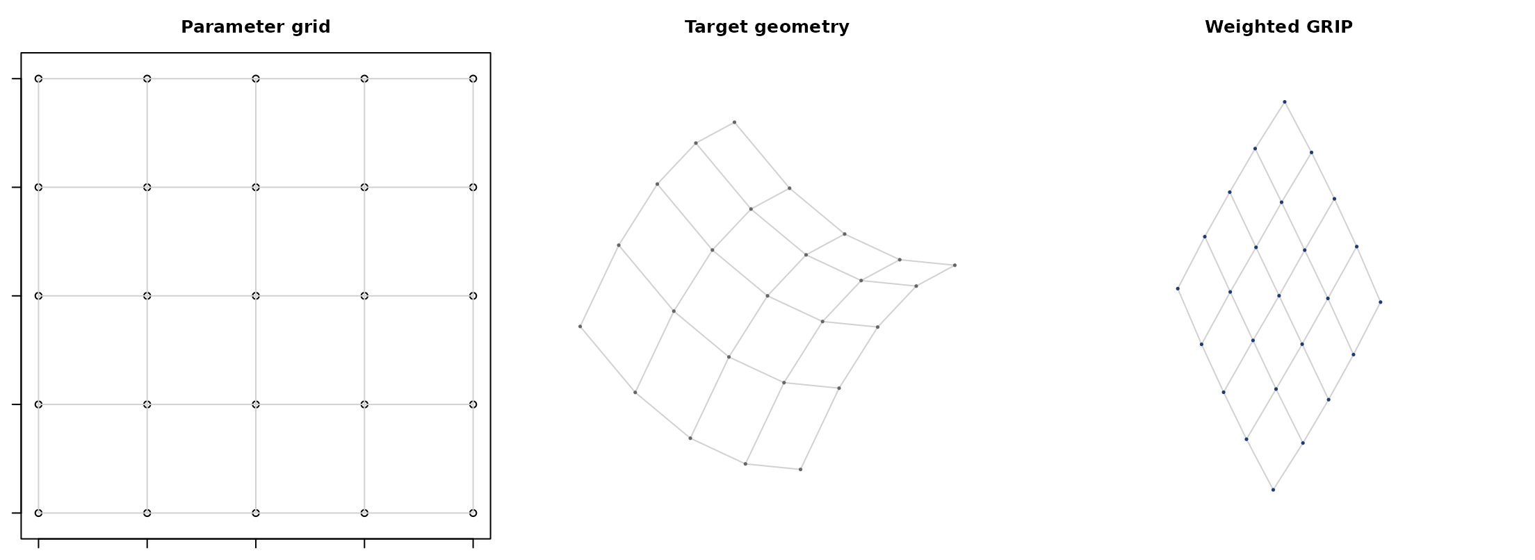
The useful design pattern here is that the topology stays simple while the metric geometry becomes nontrivial.
Wrapped surfaces
Wrapped lattices extend the same idea to periodic topologies such as a torus.
torus.graph <- torus.surface.graph(
  5, 6,
  surface = "pinched",
  minor_radius = 0.33,
  amplitude = 0.18,
  twist = 0.18
)

torus.coords <- grip(metric = "edge_length",
  torus.graph$edges,
  n = torus.graph$n,
  edge_weights = torus.graph$edge_weights,
  dim = 3,
  preset = "torus",
  seed = 2
)

knitr::kable(
  data.frame(
    family = torus.graph$family,
    surface = torus.graph$surface,
    n = torus.graph$n,
    m = nrow(torus.graph$edges)
  )
)| family | surface | n | m |
|---|---|---|---|
| torus | pinched | 30 | 60 |
plot.layout.pair(
  torus.graph$coords_surface,
  torus.coords,
  edges = torus.graph$edges,
  titles = c("Pinched torus target", "Weighted GRIP"),
  projection = "ortho",
  vertex.cols = c("#666666", "#1F3B73")
)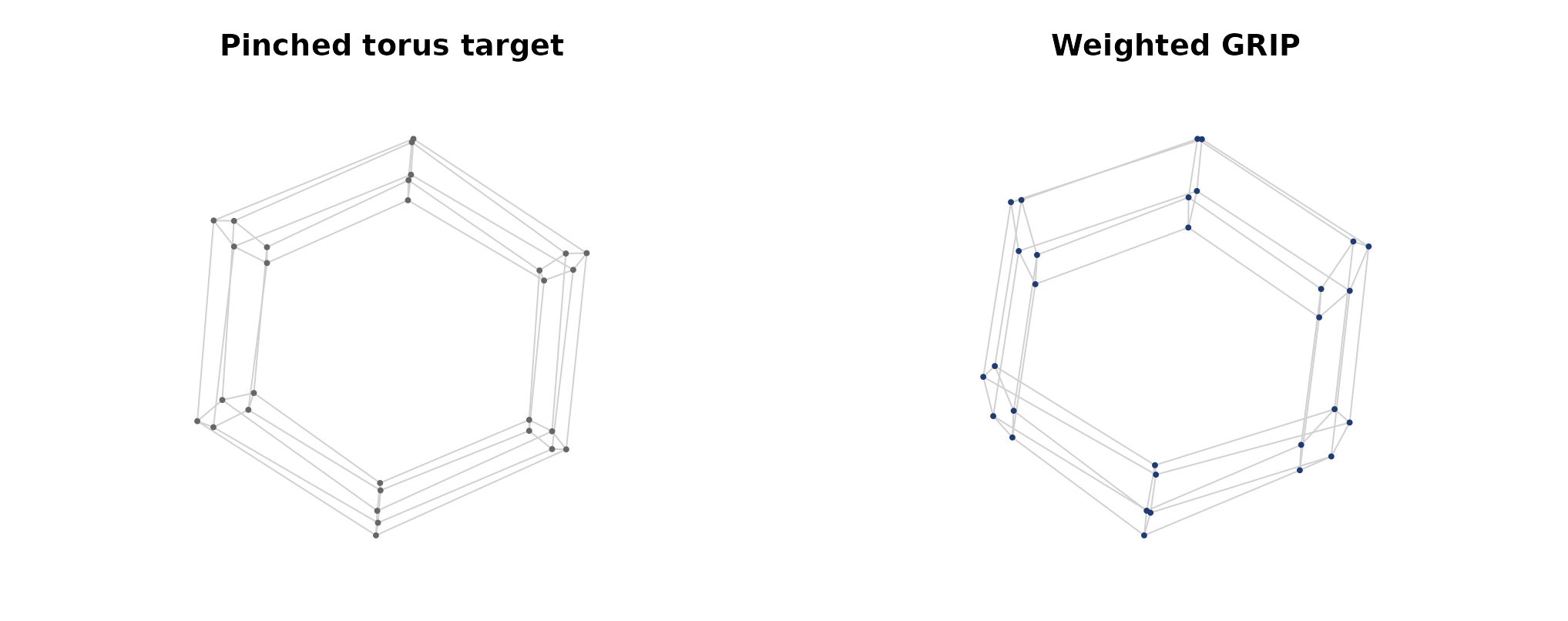
These wrapped families are especially useful when ordinary planar intuition is misleading and a 3D layout is the natural target.
Recursive and fractal families
The package now includes recursive square-mask families such as the Vicsek fractal and Sierpinski carpet variants, all of which can be lifted into curved surface geometries.
vicsek.graph <- vicsek.surface.graph(
  level = 2,
  surface = "ripple",
  amplitude = 0.55
)

vicsek.coords <- grip(metric = "edge_length",
  vicsek.graph$edges,
  n = vicsek.graph$n,
  edge_weights = vicsek.graph$edge_weights,
  dim = 3,
  preset = "carpet",
  seed = 3
)
plot.layout.pair(
  vicsek.graph$coords_surface,
  vicsek.coords,
  edges = vicsek.graph$edges,
  titles = c("Vicsek target geometry", "Weighted GRIP"),
  projection = "ortho",
  vertex.cols = c("#666666", "#1F3B73")
)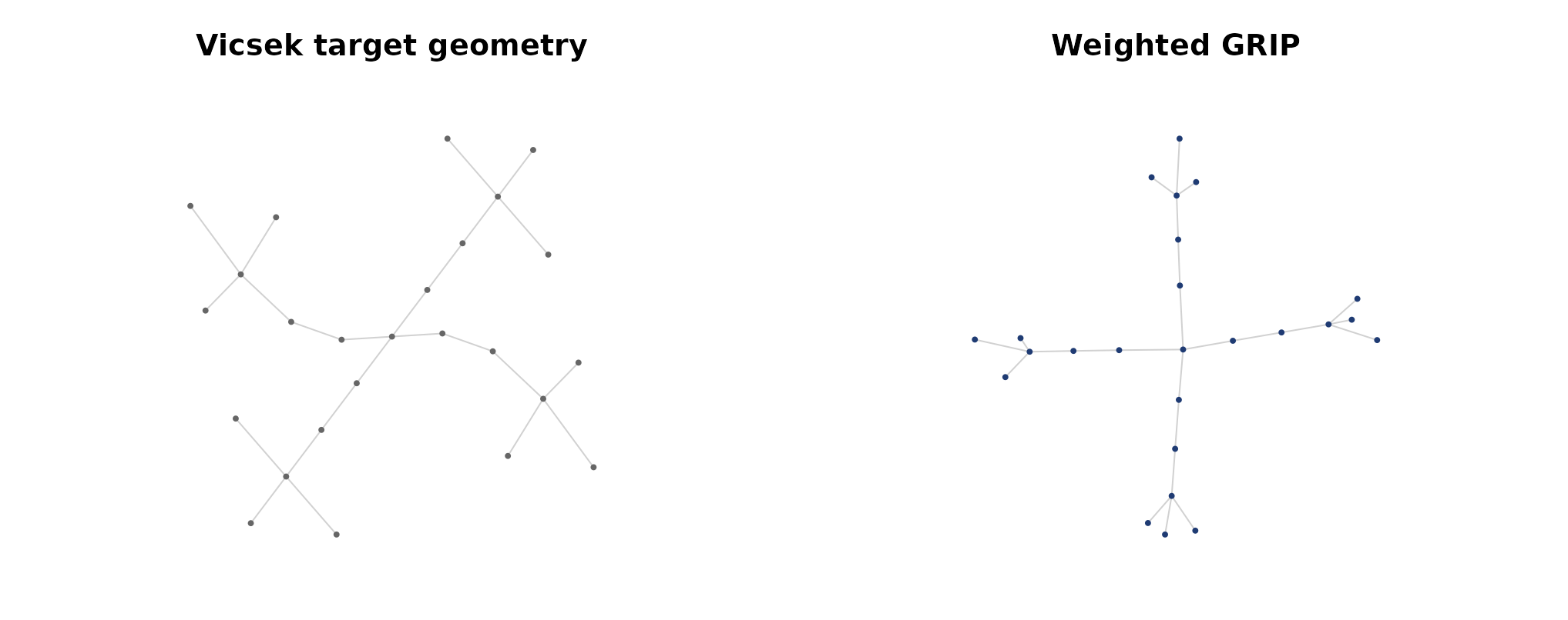
Recursive families are useful because they create holes, bottlenecks, and multi-scale detours that are hard to capture with simpler lattices.
Irregular manifolds
Not all surface families in grip are based on regular
grids. The package also includes irregular triangulated manifolds with
boundary and closed irregular surfaces.
annulus.graph <- irregular.annulus.surface.graph(
  rings = 5,
  outer_count = 24,
  inner_radius = 0.42,
  surface = "folded",
  amplitude = 0.2
)

annulus.coords <- grip(metric = "edge_length",
  annulus.graph$edges,
  n = annulus.graph$n,
  edge_weights = annulus.graph$edge_weights,
  dim = 3,
  preset = "irregular",
  seed = 4
)
plot.layout.pair(
  annulus.graph$coords_surface,
  annulus.coords,
  edges = annulus.graph$edges,
  titles = c("Irregular annulus target", "Weighted GRIP"),
  projection = "ortho",
  vertex.cols = c("#666666", "#1F3B73")
)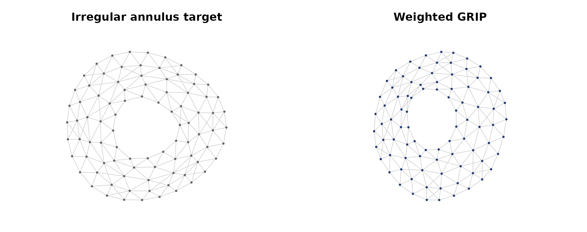
These families are important because they reduce lattice bias and produce more variable local geometry than mesh-like constructions.
Porous 3D families
The cubical branch introduces graphs that are genuinely volumetric rather than surface-like. Channel networks and related porous families create 3D geodesic detours that are hard to flatten cleanly.
cube.graph <- cube.channel.network.surface.graph(
  side = 5,
  level = 1,
  surface = "twisted",
  twist = 0.2
)

cube.coords <- grip(metric = "edge_length",
  cube.graph$edges,
  n = cube.graph$n,
  edge_weights = cube.graph$edge_weights,
  dim = 3,
  preset = "irregular",
  seed = 5
)

knitr::kable(
  data.frame(
    family = cube.graph$family,
    n = cube.graph$n,
    m = nrow(cube.graph$edges)
  )
)| family | n | m |
|---|---|---|
| cube.channel.network | 104 | 212 |
plot.layout.pair(
  cube.graph$coords_surface,
  cube.coords,
  edges = cube.graph$edges,
  titles = c("Porous cube target", "Weighted GRIP"),
  projection = "ortho",
  vertex.cols = c("#666666", "#1F3B73")
)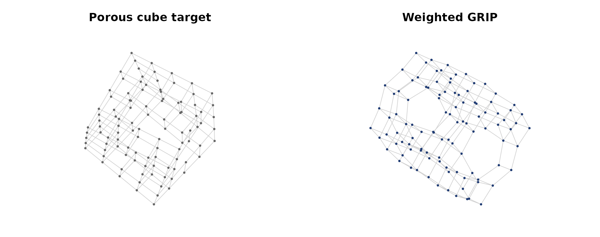
This family class is especially useful for testing whether a method can preserve large-scale volumetric structure without collapsing tunnels and channels.
Intrinsic weighted trees
Some family geometries are intrinsic rather than ambient. The weighted tree helpers preserve the exact tree topology while assigning edge lengths directly from branch-depth and branch-position rules.
tree.graph <- kary.tree.weighted.graph(
  k = 2,
  depth = 4,
  depth_rule = "geometric",
  depth_decay = 0.82,
  branch_rule = "linear",
  branch_spread = 0.25
)

tree.coords <- grip(metric = "edge_length",
  tree.graph$edges,
  n = tree.graph$n,
  edge_weights = tree.graph$edge_weights,
  dim = 2,
  preset = "tree",
  seed = 6
)

knitr::kable(
  head(tree.graph$edge_table[, c(
    "parent",
    "child",
    "child_depth",
    "branch_index",
    "edge_weight"
  )]),
  digits = 3
)| parent | child | child_depth | branch_index | edge_weight |
|---|---|---|---|---|
| 1 | 2 | 1 | 1 | 1.411 |
| 1 | 3 | 1 | 2 | 1.814 |
| 2 | 4 | 2 | 1 | 1.157 |
| 2 | 5 | 2 | 2 | 1.487 |
| 3 | 6 | 2 | 1 | 1.157 |
| 3 | 7 | 2 | 2 | 1.487 |
plot.layout(
  tree.coords,
  tree.graph$edges,
  main = "Intrinsic weighted tree",
  vertex.col = "#1F3B73",
  edge.col = "gray80",
  pch = 16,
  cex = 0.6
)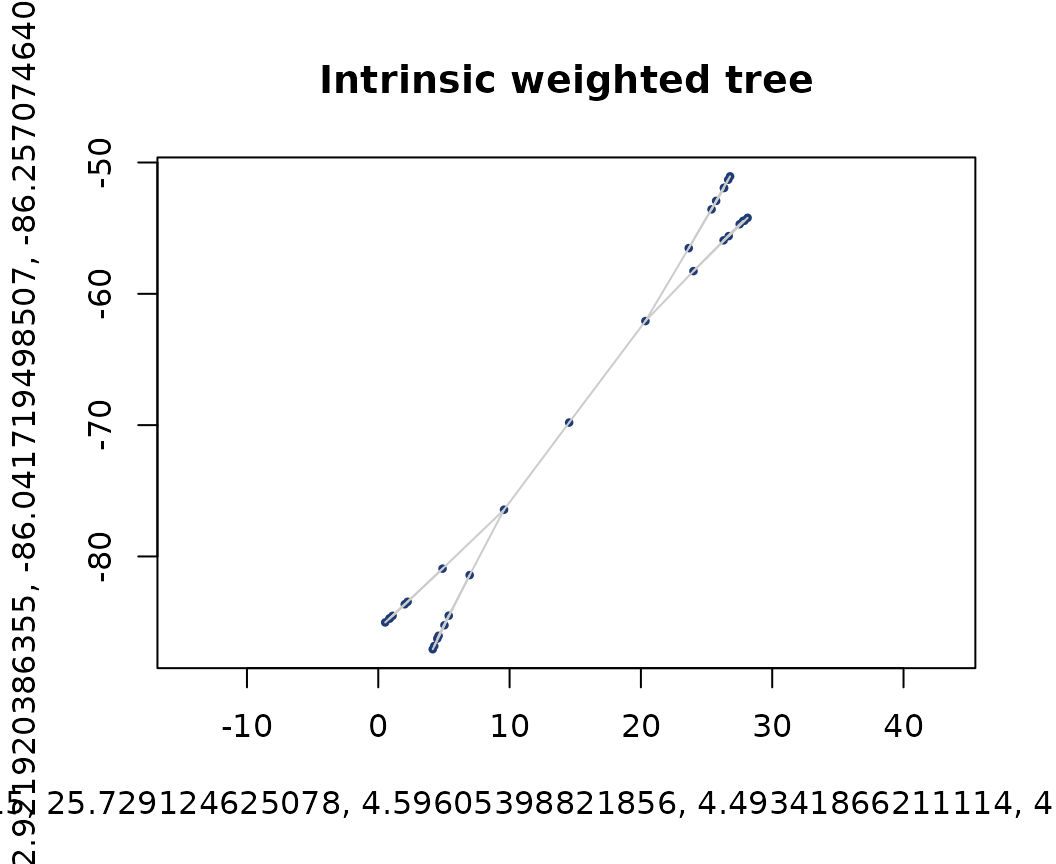
These tree families are useful because they separate intrinsic weighted geometry from any arbitrary 3D embedding choice.
Why this family library matters
The family collection now serves three roles:
- it gives users concrete examples of what the package can represent,
- it supports regression testing and benchmark design,
- and it makes it possible to study layout behavior under controlled geometric variation rather than only on a handful of fixed toy graphs.
Learn more
-
Getting Started with gripintroduces the main layout APIs. -
Weighted Graph Layouts with gripexplains how to use these family bundles with the weighted sister API. -
Interactive Exploration with gripuishows how to browse the larger family registry throughrun_gripui_family().