Getting Started with grip

What this vignette covers

grip has four main user workflows:

• grip() for ordinary unweighted or topology-first graphs,
• weighted.grip() when edge lengths carry geometry you want to keep,
• compare.layouts() and score.layout() when you want a disciplined real-data shortlist,
• trace.grip() and trace.weighted.grip() when you need diagnostics rather than just a final picture.

This vignette is the shortest path through the default workflow. It shows how to:

• compute a first unweighted layout,
• score it,
• compare a few plausible candidates,
• and decide when to switch to the specialist guides.

For weighted layouts, real-data search, tracing, and interactive exploration, the later guides go deeper. Advanced GKK/LGKK tools are public, but they are treated as later-stage experimental helpers rather than the default starting point.

library(grip)

A first unweighted layout

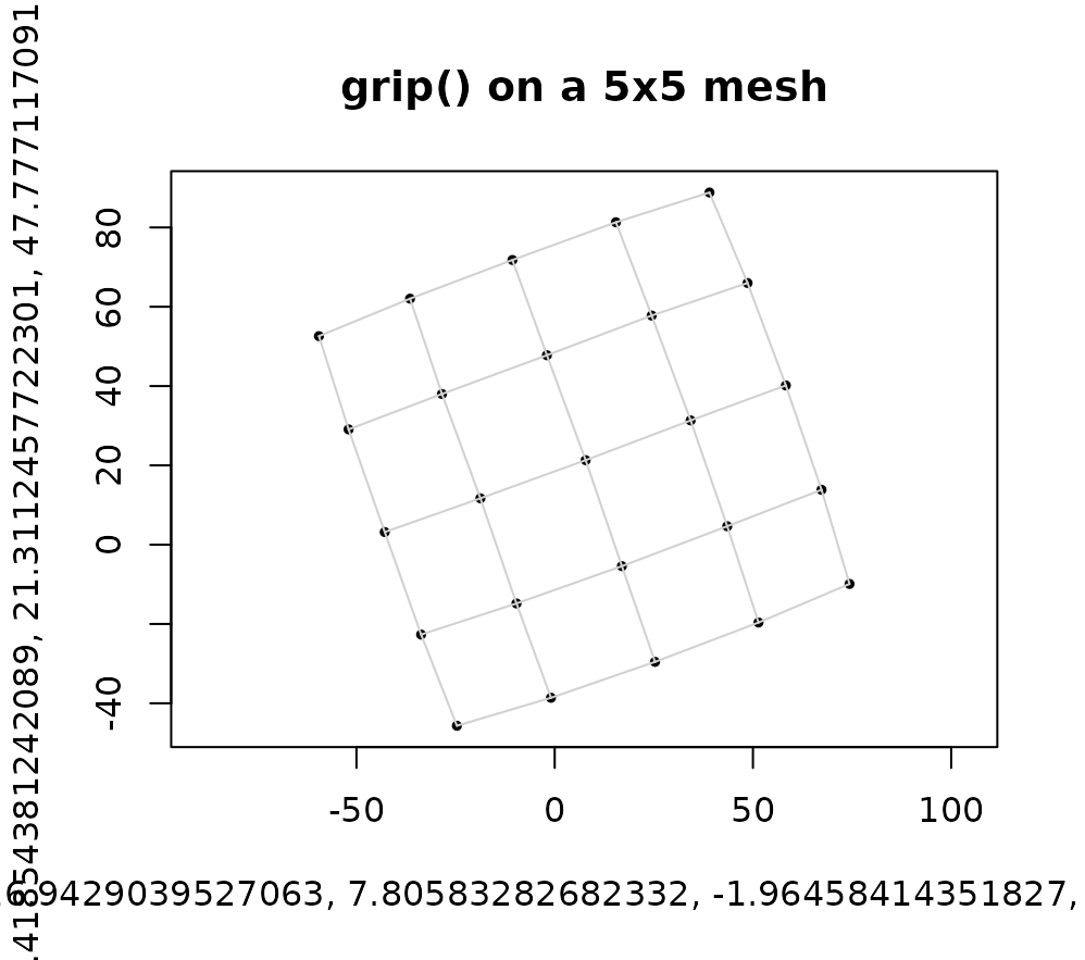
For an ordinary unweighted graph, grip() is the default starting point. Here is a small mesh in 2D.

mesh.edges <- edges.mesh(5, 5)
mesh.coords <- grip(
  mesh.edges,
  n = 25,
  dim = 2,
  preset = "mesh",
  seed = 1
)

mesh.score <- score.layout(mesh.coords, edges = mesh.edges, n = 25)
knitr::kable(mesh.score[, c(
  "sampled.stress",
  "edge.length.cv",
  "sampled.nonedge.sep.ratio"
)], digits = 3)

sampled.stress	edge.length.cv	sampled.nonedge.sep.ratio
9.19	0.055	1.286

plot.layout(
  mesh.coords,
  mesh.edges,
  main = "grip() on a 5x5 mesh",
  pch = 16,
  cex = 0.65,
  edge.col = "gray82"
)

For small and medium unweighted graphs, that is often all you need:

• choose dim = 2 or dim = 3,
• optionally start from a preset,
• and score or compare a few candidate settings if the graph is important.

Compare a few plausible candidates

If the first picture matters, it is usually better to compare a short candidate list than to tune blindly. compare.layouts() runs several seeds and summarizes the results in a score table.

mesh.cmp <- compare.layouts(
  edges = mesh.edges,
  n = 25,
  dim = 2,
  candidates = c("default", "mesh", "tree"),
  seeds = 1:2,
  sample.size.stress = 500L,
  sample.size.nonedge = 1000L,
  edge.crossings = "never"
)

knitr::kable(mesh.cmp$summary[, c(
  "candidate",
  "sampled.stress.mean",
  "edge.length.cv.mean",
  "sampled.nonedge.sep.ratio.mean",
  "score.composite"
)], digits = 3)

candidate	sampled.stress.mean	edge.length.cv.mean	sampled.nonedge.sep.ratio.mean	score.composite
mesh	9.192	0.055	1.289	0.194
tree	1.790	0.321	0.233	0.528
default	18.721	0.166	0.247	0.778

That same pattern scales to real graphs:

• shortlist a few plausible presets,
• run several seeds,
• inspect the summary table before choosing a favorite picture,
• then search locally only if the graph is important enough to justify it.

What if the graph is weighted?

If a graph has edge weights but those weights are mostly metadata, a topology-first grip() run can still be a useful baseline. When the edge lengths represent geometry that the layout should preserve, the default path changes:

• start from weighted.grip(),
• prefer 3D when the graph geometry is genuinely three-dimensional,
• and add GKK/LGKK only later if you need advanced geodesic-aware scoring or polish on a smaller weighted candidate set.

When should you switch workflows?

Start with grip() when the graph is fundamentally unweighted and you mainly care about its combinatorial structure.

Switch to the other guides when the task changes:

• use weighted.grip() when edge lengths encode geometry you care about,
• use compare.layouts() on real graphs when you want a disciplined shortlist rather than a single run,
• use trace.grip() or trace.weighted.grip() when you want to inspect how a solve evolves,
• use GKK/LGKK only after you already have weighted candidate layouts and need advanced experimental geodesic-aware scoring or polish,
• use run_gripui() or run_gripui_family() in an interactive R session when you want app-based exploration.

Where to go next

• Weighted Graph Layouts with grip covers weighted solving, geodesic scoring, and 2D-versus-3D decisions.
• Choosing Layouts for Real Data focuses on candidate shortlisting, local search, and real-data evaluation.
• Tracing and Diagnosing Layouts covers trace objects and per-frame diagnostics.
• Interactive Exploration with gripui is a website article about the package’s Shiny tools.
• Synthetic Graph Families and Geometries is a website article about the benchmark and geometry library.