What does a 3D embedding preserve?

Three decisions, three different questions

A 3D picture combines a representation of the observations, a distance rule, and a fitted approximation. Separating these decisions prevents a visually striking plot from becoming its own evidence.

Here we hold the observations fixed and compare L1 normalization with Euclidean distance, max normalization with Euclidean distance, and max normalization with L-infinity distance. We measure each fit against its own original-space distances. We do not compare ecological validity.

The linf corner-geometry article explains how normalization alone can separate directions away from a dominant taxon. This companion asks how much of the chosen distance geometry survives an additional reduction to three dimensions.

What is fitted, and what counts as success?

We use two examples: 48 reproducible four-part synthetic compositions and a seeded sample of 300 distinct compositions from the 2,000 observations in linf::valencia2k. The latter is a stratified teaching subset of VALENCIA data, not a population-prevalence sample. See the dataset guide. All 178 taxon columns are retained. One distinct composition is one fit row; no participant weighting or clinical outcome enters the analysis.

For each example and target, we fit three dimensions using metric.mds() with the SGD backend, inverse-squared target-distance weights, 300 full pair passes, and seeds 11, 29 and 47. Each seed gives one random start. The Zheng schedule uses schedule.epsilon=0.01; checkpoints occur every ten passes. The lowest achieved objective among these three runs supplies the illustration. All seed results are reported, including budget exhaustion; none is called a certified optimum.

There are only 44,850 empirical pairs, so these examples use full distance matrices and exact all-pairs evaluation. This is a teaching choice, not a prescription for large datasets. See the sparse fitting guide for larger collections.

The primary diagnostic is

$E=100\sqrt{\frac{1}{|\mathcal P|} \sum_{(i,j)\in\mathcal P}\left(\frac{d_{ij}-\delta_{ij}}{\delta_{ij}}\right)^2}, \qquad d_{ij}=\|y_i-y_j\|_2.$

Here $\delta_{ij}>0$ is the selected target distance, $y_i$ is a fitted 3D coordinate, and $\mathcal P$ contains all unordered pairs of distinct fit rows. Zero means exact reproduction; 10% means an RMS relative error of 0.10, not that every distance is accurate to 10%. No additional scale is fitted when calculating this diagnostic. The solver’s returned coordinates already include its documented objective-based scale adjustment.

There is no universal acceptable percentage. A successful evaluation computes the stated quantity correctly, reveals where errors occur, and exposes seed sensitivity. A lower value for one target family does not show that its normalization or metric is scientifically better than another.

Construct the targets explicitly

For nonnegative rows with positive total, let $p=x/\sum_jx_j$ and $q=x/\max_jx_j$ . The targets are respectively $\|p_i-p_j\|_2$ , $\|q_i-q_j\|_2$ , and $\|q_i-q_j\|_\infty=\max_k|q_{ik}-q_{jk}|$ . Max normalization and L-infinity distance are separate operations.

P <- X / rowSums(X)
Q <- X / apply(X, 1, max)
D1 <- as.matrix(dist(P))
D2 <- as.matrix(dist(Q))
D3 <- as.matrix(dist(Q, method = 'maximum'))
fit <- metric.mds(distance.matrix=D3, dim=3, backend='sgd',
  pair.weights='inverse_squared', init='random', n.init=1,
  max.iter=300, seed=11,
  sgd.control=list(scheduler='zheng',schedule.epsilon=.01,checkpoint.every=10))

distance.matrix uses these values directly: no neighbor graph or shortest paths replace them. Remove duplicate normalized rows before using inverse-squared weights, and retain the mapping back to original observations. Near-zero positive targets are retained, not floored; they can make relative error demanding. In this empirical subset, the smallest positive target in each family is:

knitr::kable(data.frame(Method=names(targets),Minimum=vapply(targets,
  function(D) min(D[lower.tri(D)]),numeric(1))),digits=6,row.names=FALSE)

Method	Minimum
L1 / Euclidean	0.000578
Max / Euclidean	0.000494
Max / L-infinity	0.000309

A small example with a known reference

Four-part L1 compositions lie in a three-dimensional affine hyperplane, so their Euclidean distances admit an exact 3D representation. We can construct one directly using an orthonormal basis, independent of MDS. Max-normalized points can span several faces in four dimensions, and L-infinity targets need not be Euclidean even before reducing dimension.

H<-qr.Q(qr(cbind(rep(1,4),diag(4)[,1:3]))) [,-1,drop=FALSE]
exact<-z$toy%*%H
exact.error<-study_score(exact,toy.targets[[1]])[1]
stopifnot(exact.error<1e-10)
knitr::kable(toy$scores[,1:6],digits=3,row.names=FALSE,
  col.names=c("Method","Seed","RMS (%)","Short (%)","Long (%)","Median absolute (%)"))

Method	Seed	RMS (%)	Short (%)	Long (%)	Median absolute (%)
L1 / Euclidean	11	0.000	0.000	0.000	0.000
L1 / Euclidean	29	0.000	0.000	0.000	0.000
L1 / Euclidean	47	0.000	0.000	0.000	0.000
Max / Euclidean	11	8.643	8.900	8.286	3.991
Max / Euclidean	29	8.643	8.897	8.288	3.990
Max / Euclidean	47	8.643	8.899	8.288	3.984
Max / L-infinity	11	14.625	12.825	15.160	9.782
Max / L-infinity	29	14.625	12.823	15.164	9.791
Max / L-infinity	47	14.625	12.829	15.161	9.799

The independently constructed exact L1 representation has RMS relative error below $10^{-10}$ percent. Any larger error in the fitted L1 rows above is optimization error under this budget. For the other targets, an observed residual can combine dimensional incompatibility and optimization error; these runs do not separate the two or establish the best achievable stress.

Results on the bundled microbiome example

knitr::kable(real$scores[,1:6],digits=2,row.names=FALSE,
  col.names=c("Method","Seed","RMS (%)","Short (%)","Long (%)","Median absolute (%)"))

Method	Seed	RMS (%)	Short (%)	Long (%)	Median absolute (%)
L1 / Euclidean	11	13.07	13.31	7.12	5.27
L1 / Euclidean	29	13.07	13.28	7.11	5.22
L1 / Euclidean	47	12.91	13.22	7.23	5.45
Max / Euclidean	11	14.86	10.93	18.64	6.98
Max / Euclidean	29	14.79	10.81	18.79	6.82
Max / Euclidean	47	14.97	11.03	18.22	7.07
Max / L-infinity	11	19.67	13.53	20.51	11.04
Max / L-infinity	29	19.66	13.42	20.38	11.20
Max / L-infinity	47	19.73	13.59	20.55	11.32

The best observed RMS errors are 12.91%, 14.79%, 19.66%, in the method order shown above. These are achieved errors for different target families, not a ranking of biological usefulness. All 18 runs (both examples) ended at the iteration limit. Values printed as zero are rounded, not a claim of exact numerical equality.

The columns for shortest and longest distances use each target’s own bottom and top distance deciles, including boundary ties. Their membership can differ between target families. Every fit is checked against every pair; this measures training-distance fidelity, not generalization to unseen samples.

op<-par(mar=c(8,4,1,1))
plot(NA,xlim=c(.6,3.4),ylim=range(c(0,real$scores$RMS_percent)),xaxt='n',
     xlab='',ylab='RMS relative error (%)')
axis(1,1:3,names(targets),las=2)
for(i in 1:3) points(rep(i,3)+c(-.08,0,.08),real$scores$RMS_percent[real$scores$Method==names(targets)[i]],
  pch=16,col=c('#0072B2','#D55E00','#009E73')[i])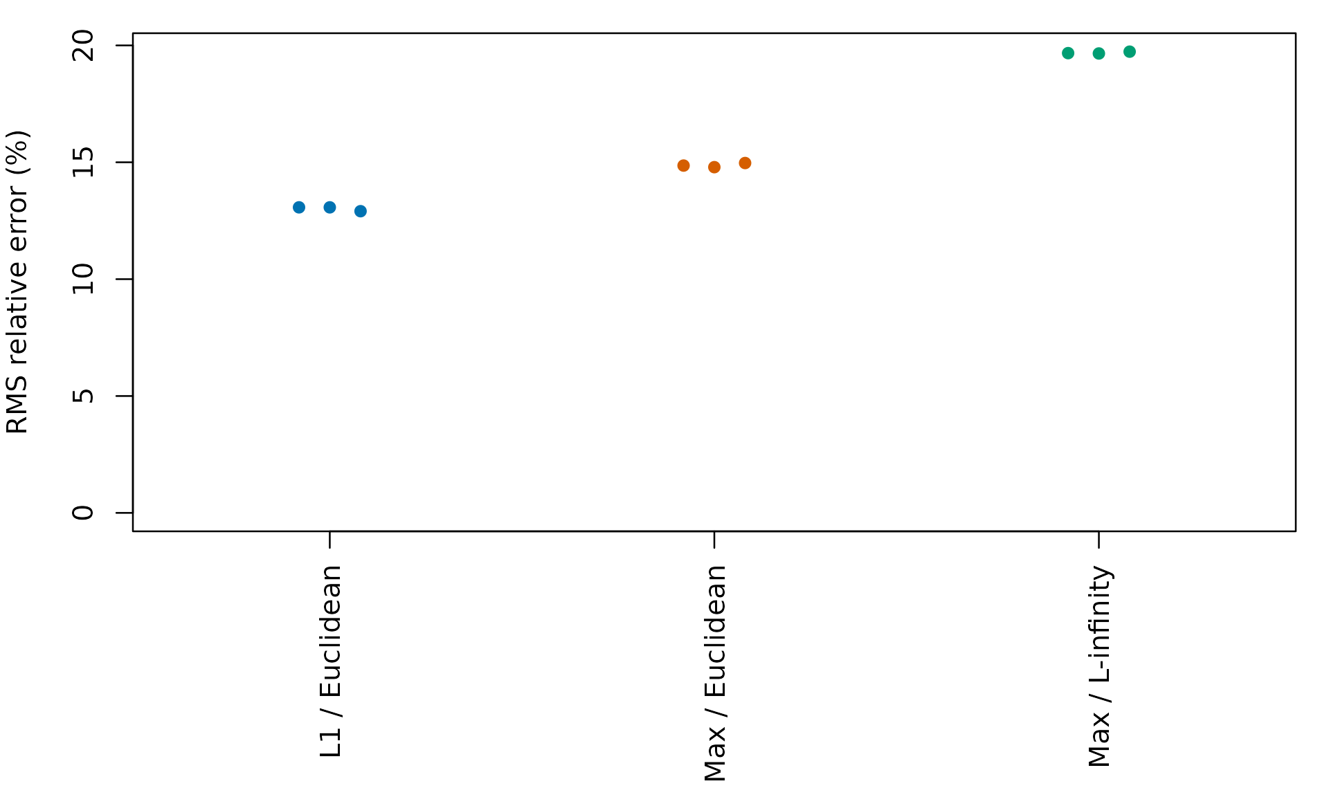

Each point is one recorded seed. Lower is better only relative to the target family on the same axis; differences between methods also reflect different distance geometries.

par(op)

Where are distances distorted?

The following plots use the best of the three recorded starts for each method. Every empirical pair is shown. The diagonal is exact preservation; vertical spread indicates errors hidden by a single RMS number.

op<-par(mfrow=c(1,3),mar=c(4,4,3,1))
for(m in names(targets)) {
  t<-as.numeric(as.dist(targets[[m]])); d<-as.numeric(dist(real$best[[m]]$coords))
  lim<-range(c(0,t,d))
  plot(t,d,pch=16,cex=.2,col=adjustcolor('#0072B2',alpha.f=.12),
       xlim=lim,ylim=lim,asp=1,main=m,xlab='Target distance',ylab='3D distance')
  abline(0,1,col='#D55E00',lwd=2)
}

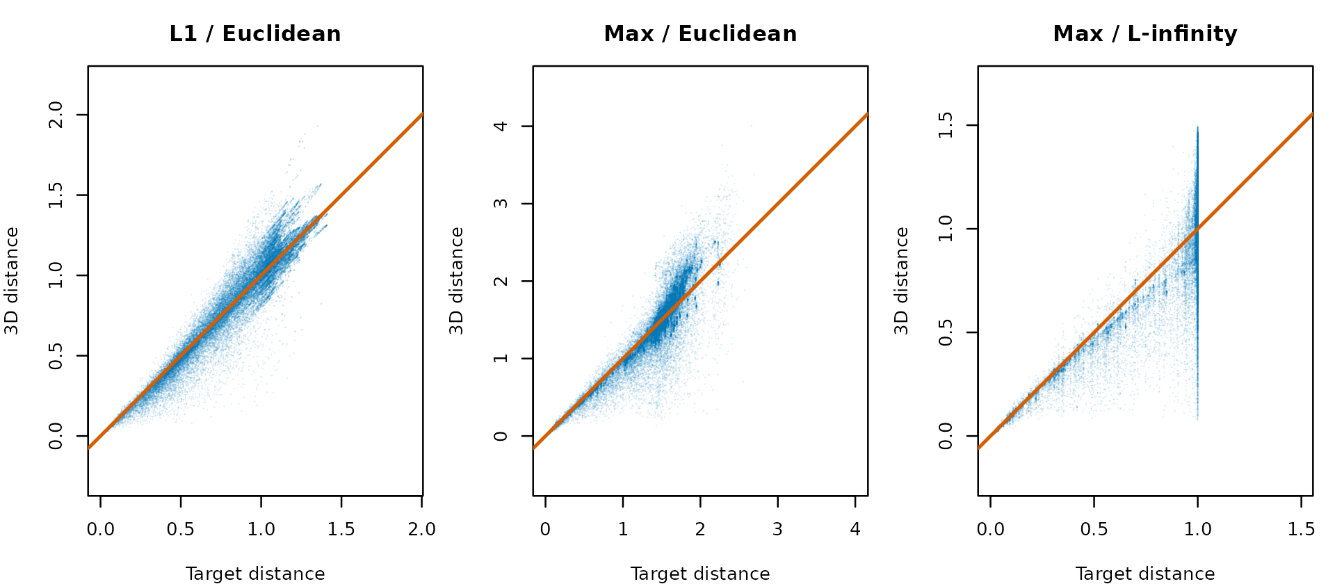
Target distance versus fitted Euclidean distance in 3D, in each target’s own units. Axes within each panel have the same range.

par(op)

Explore the three fitted views

Drag to rotate and scroll to zoom. All views use the same observations, colors, sphere radius, camera and coordinate limits. We remove translation and align orientations to the first fit using an orthogonal transformation; we do not rescale the drawings. Alignment preserves all fitted pair distances and cannot remove deformation. Axes are arbitrary embedding coordinates. Different overall sizes may reflect different target-distance units.

L1 normalization, Euclidean distance

L1 / Euclidean — best of three recorded full SGD fits

Max normalization, Euclidean distance

Max / Euclidean — best of three recorded full SGD fits

Max normalization, L-infinity distance

Max / L-infinity — best of three recorded full SGD fits

A visible arm or gap is a feature to investigate in the original data and selected targets. It is not, by itself, evidence of a community boundary. Colors describe the original dominant taxon; changing normalization or fitting does not reassign these labels.

Reproduce and interpret the comparison

This is a website article for the development version of grip with direct distance.matrix support. It requires linf’s bundled data and ivue/rgl for interactive figures. The source-visible embedding-study.R beside this article contains data selection, scoring, fitting, and alignment functions. From a source checkout, run make embedding-fidelity-vignette. The on-demand renderer records source fingerprints, session information, selected rows and every fit’s settings; cached fits are keyed by inputs, solver settings and implementation fingerprints. It does not publish the site.

The article reports the specified 300-pass experiment without extending runs until a preferred picture appears. More starts or longer schedules would be new experiments. The examples do not determine an optimal normalization, certify convergence, or provide participant-level uncertainty estimates.