Comparing SGD and SMACOF for metric MDS

What is being compared?

metric.mds() fits Euclidean coordinates to graph shortest-path distances. Its default backend = "sgd" uses native stochastic gradient descent (SGD), based on Zheng, Pawar and Goodman (2018), with the default learning-rate schedule following Hangan, Kobourov and Miller (2026). SGD visits pairs of points in a randomly shuffled order, moving each pair closer together or farther apart to better match its target distance. These changes take effect immediately, and the learning-rate schedule reduces the size of the adjustments as fitting proceeds.

The alternative backend = "smacof" uses the optional smacof package (Mair, Groenen and de Leeuw, 2022). SMACOF combines information from all pairs before updating the entire configuration at once. Each update is designed to reduce total stress; an individual SGD adjustment need not reduce total stress, even though it improves the distance for the pair being adjusted. With the default pair.weights = "uniform", both minimize the same raw distance stress:

$$S(Z) = \sum_{i<j} \bigl(\lVert z_i-z_j\rVert-d_{ij}\bigr)^2.$$

Both also support pair.weights = "inverse_squared", the graph-drawing weighting used by Zheng, Pawar and Goodman (2018). The weighting comparison below shows how this changes the fitted layouts. The original 420-fit comparison uses uniform weighting throughout.

This is a comparison of these implementations and settings on small synthetic examples. For a more extensive comparison of SGD and SMACOF across 18 benchmark datasets, see Hangan, Kobourov and Miller (2026), who compare their SGD solver with scikit-learn’s SMACOF implementation.

The figure labels and plots use normalized error, $\sqrt{S(Z)/\sum_{i<j}d_{ij}^2}$. Lower is better; zero means exact agreement with the target distances. Within a dataset, its ranking is identical to raw stress. Raw stress is also reported. We recompute both from the returned coordinates, rather than compare differently normalized backend reports.

The precomputed experiment uses 14 datasets, five paired starts, three allowances, and two backends: 420 planned fits. Every example is displayed below, including both cloud sizes. Except for the planar control, all fits and interactive views are three-dimensional. The plane is fitted and plotted in two dimensions.

A small, executable example

Construct a saddle over $[-1,1]^2$, with $z=0.8(x^2-y^2)$. This is a two-dimensional surface embedded in 3D. To compare ambient distances, represent the cloud as a complete graph with Euclidean edge lengths. The triangle inequality then makes graph shortest-path distances equal to the original Euclidean distances.

library(grip)
source(system.file('scripts', 'metric-mds-comparison.R', package = 'grip'), local = TRUE)
grid <- seq(-1, 1, length.out = 5)
uv <- as.matrix(expand.grid(x = grid, y = grid))
X <- cbind(uv, z = .8 * (uv[, 1]^2 - uv[, 2]^2))
edges <- t(combn(nrow(X), 2))
lengths <- sqrt(rowSums((X[edges[, 1], ] - X[edges[, 2], ])^2))
prepared <- prepare.graph.geodesic.mds(edges = edges, n = nrow(X),
                                      edge.weights = lengths)
start <- withr::with_seed(11, matrix(rnorm(nrow(X) * 3), nrow(X), 3))
# Schedule completion emits an iteration-limit warning, not convergence.
sgd <- suppressWarnings(metric.mds(prepared = prepared, dim = 3,
  init = start, n.init = 1, max.iter = 30, seed = 11, diagnostics = FALSE))
sgd$metadata$engine  # "sgd": backend omitted deliberately
#> [1] "sgd"
sgd$metadata$termination
#> [1] "iteration_limit"
smacof.fit <- NULL
if (requireNamespace('smacof', quietly = TRUE)) {
  smacof.fit <- suppressWarnings(metric.mds(prepared = prepared, dim = 3,
    init = start, n.init = 1, max.iter = 30, seed = 11,
    backend = 'smacof', eps = 1e-8, diagnostics = FALSE))
  rbind(SGD = comparison_score(sgd$coords, prepared$distance_matrix),
        SMACOF = comparison_score(smacof.fit$coords, prepared$distance_matrix))
}
#>         raw_stress      error
#> SGD     0.06260239 0.00904617
#> SMACOF 20.38613660 0.16324382

This introductory 25-point fit is separate from the timing experiment. Its coordinates are also shown: the timing labels below belong only to the saved experiment, not to this run during document generation.

small.case <- comparison_cases(5L)[['saddle-25']]
small.fits <- list(sgd = list(coords = sgd$coords),
  smacof = list(coords = if (!is.null(smacof.fit)) smacof.fit$coords else NULL))
if (have.ivue) {
  comparison_view(small.case, small.fits)
} else {
  # A 3D projection of this run; precomputed experiment images below use ivue.
  Z <- cbind(small.case$X[,1], small.case$X[,2], small.case$X[,3])
  Zs <- comparison_align(sgd$coords, Z)
  view <- function(A) cbind(.8*A[,1] - .6*A[,2], .3*A[,1] + .4*A[,2] + .866*A[,3])
  all <- rbind(Z, Zs)
  colors <- rep(c('gray55','#1769AA'), each = nrow(Z))
  if (!is.null(small.fits$smacof$coords)) {
    all <- rbind(all, comparison_align(small.fits$smacof$coords, Z))
    colors <- c(colors, rep('#D66A19', nrow(Z)))
  }
  plot(view(all), asp = 1, pch = 16, col = colors,
       xlab = '3D projection: horizontal', ylab = '3D projection: vertical')
}

Saddle 25 points; Ambient Euclidean targets. Gray: reference; blue: SGD; orange: SMACOF. Rigid alignment only.

The executable 25-point saddle example: gray reference, blue SGD, orange SMACOF (when available). Both fits use the same starting coordinates and 30 passes/iterations.

max.iter defaults to 1000; 30 is an explicit short trial allowance. One SGD pass visits all unordered pairs. One SMACOF iteration is a different operation, so equal iteration counts are not equal work. SGD’s schedule ends with iteration_limit, even when it returns an earlier, better checkpoint. SMACOF may stop earlier using eps; this tolerance must not be passed to SGD. The learning-rate defaults are provisional calibration choices.

Datasets and timing protocol

The plane, paraboloid and saddle use regular 8-by-8 and 12-by-12 grids on $[-1,1]^2$, giving 64 and 144 vertices. Their lifts are, respectively, $z=0$, $z=0.8(x^2+y^2)$, and $z=0.8(x^2-y^2)$. The Gaussian clouds have three independent standard-normal coordinates with fixed seeds. The spatial graph follows a helix $(\cos t,\sin t,t/\pi)$, $0\leq t\leq3\pi$, with edges between consecutive vertices and between vertices seven indices apart. Every graph edge is weighted by its Euclidean length in the generating coordinates.

For the paraboloid and saddle, two target definitions are compared:

• Ambient Euclidean: all straight-line distances in the generating 3D cloud, represented by a complete weighted graph. An exact 3D realization exists; classical MDS provides a useful numerical check.
• Local graph paths: shortest paths on the grid with horizontal, vertical, and both diagonal connections. These are exact distances for that finite graph, not exact geodesic distances on the continuous quadform. They depend on sampling and allowed directions. Small graph-distance stress need not reconstruct the generating surface.

The helix uses local graph-path targets. Its generating coordinates are a reference drawing, not a guaranteed exact realization of all graph distances. The reference mesh on each quadform connects corresponding sampled vertices; it is a display aid, not a geodesic or surface-recovery certificate.

For every dataset, both backends receive the same saved starting-coordinate recipe, for seeds 1–5, and n.init = 1. Each allowance of 10, 30 or 100 starts a separate fit from those coordinates. SGD uses the hybrid schedule with initial rate 0.5, boundary rate 0.01, switch fraction 0.4, and scoring after every pass; SMACOF uses eps = 1e-8. Backend order alternates between paired blocks. No setting was chosen from the observed winners.

Elapsed fitting time includes the wrapper, target normalization, optimization, and checkpoint scoring. Shared graph preparation, process startup, namespace loading, independent final scoring, alignment, and rendering are excluded. The two namespaces are loaded before timing either backend. Each fit runs in an isolated process with a 30-second allowance; the full experiment has a 1,800-second allowance. Errors and timeouts remain in the result table and are not replaced by successful reruns. These are provisional workload limits.

The plots show median time and median normalized error across five starts, with horizontal and vertical interquartile ranges. Numeric labels identify the allowances. Each marker is a separate restarted experiment, not a checkpoint on one optimization trajectory. There is no retrospective best-of-three selection. Values below 0.001 seconds or error below $10^{-12}$ are clipped only for logarithmic plotting; the tables retain measured values.

knitr::kable(as.data.frame(table(Backend = rows$backend, Status = rows$status)),
             col.names = c('Backend','Outcome','Fits'))

Backend	Outcome	Fits
sgd	ok	210
smacof	ok	210

knitr::kable(do.call(rbind, lapply(split(rows, rows$backend), function(z) {
  data.frame(Backend = z$backend[1], Fits = nrow(z),
    `Successful fits` = sum(z$status == 'ok'),
    `Total fit seconds` = sum(z$seconds, na.rm = TRUE),
    `Total worker seconds` = sum(z$worker_seconds), check.names = FALSE)
})), row.names = FALSE, digits = 3)

Backend	Fits	Successful fits	Total fit seconds	Total worker seconds
sgd	210	210	7.441	273.481
smacof	210	210	5.173	268.876

At the largest allowance (100 passes/iterations), SGD has lower normalized error in 69 of 70 completed pairs, and SMACOF in 1; differences no larger than $10^{-10}$ count as ties. This compares a specified iteration allowance, not equal elapsed time. Across all three allowances, total recorded fitting time is 7.441 seconds for SGD and 5.173 for SMACOF. These examples favor SGD’s achieved accuracy but do not establish a universal speed advantage. Use the per-example plots to examine the trade-off.

An ok outcome means a fit returned usable coordinates; it does not mean convergence. Figure tables below report the actual pass/iteration count and termination reason. Worker time includes startup and communication and is reported separately. For a forcibly stopped worker, fitting time may be unavailable; summing recorded fitting time alone would then understate total effort. Timing is machine-dependent, especially for these small examples. This run used a shared workstation without CPU isolation; short timings are sensitive to background activity and timer resolution.

How to read the embedding figures

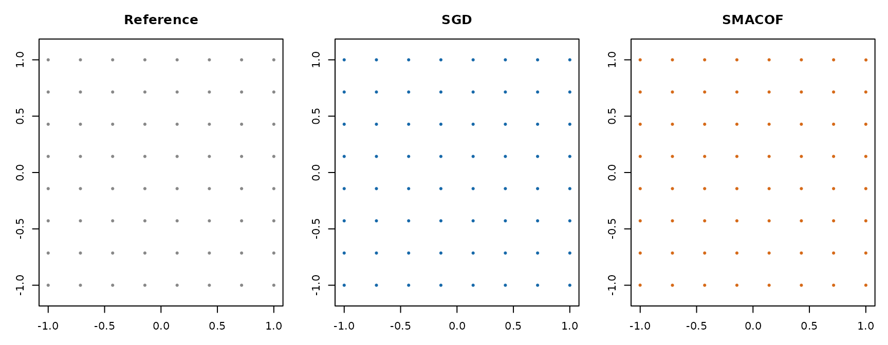
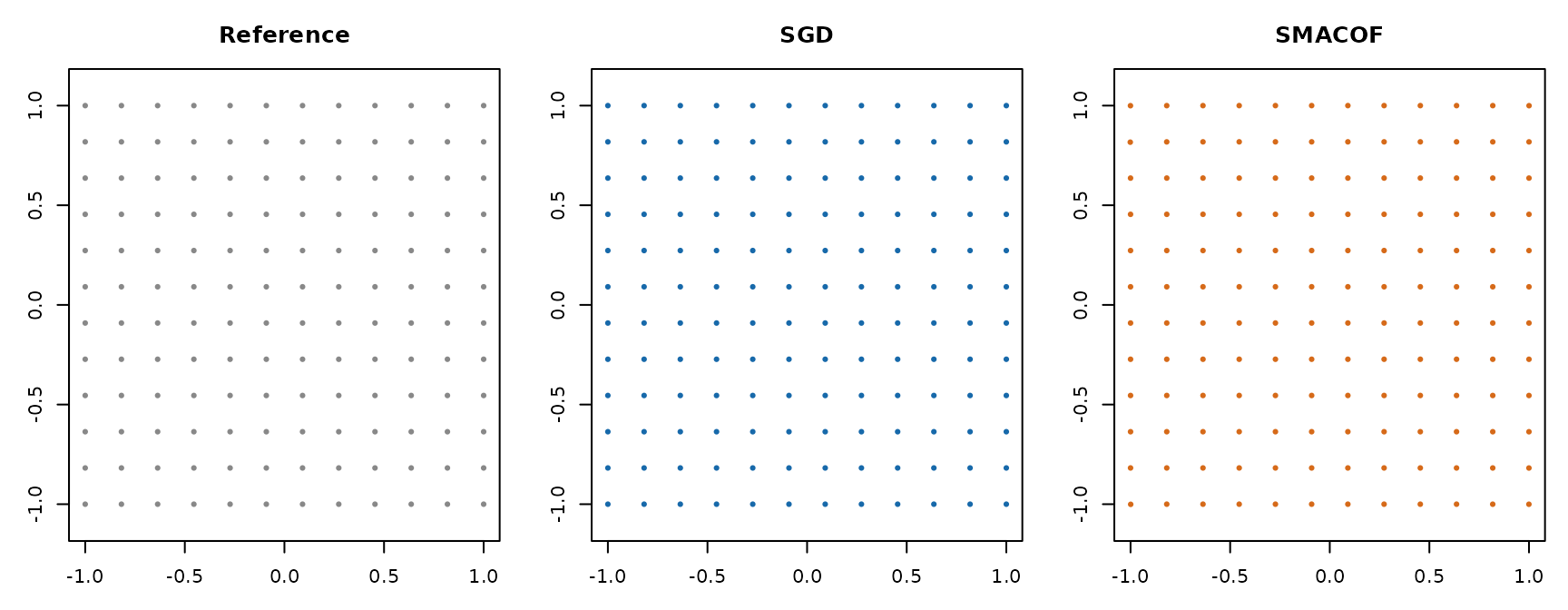
Gray is the generating reference; blue is SGD; orange is SMACOF. Each saved experiment figure shows seed 1 and allowance 100, selected in advance and identically for both backends. It is not the best seed or the fit nearest the median. A failed selected run stays unavailable. Figure tables report that exact run’s error, raw stress and fitting time, as well as a separately computed classical-MDS reference.

Except for the two local-graph saddle examples described below, we center each fit, then apply an orthogonal rotation/reflection to match corresponding reference vertices. No rescaling is performed for alignment. The reported scores use original returned coordinates. These operations preserve all fitted distances; shared axes retain the input units. Blue and orange graph segments show the same edges in each embedding. Dense complete graphs are shown as clouds, avoiding thousands of overlapping edges.

The two Saddle: Local graph paths examples use surface-shape alignment. This display matches nearby surface locations without requiring their vertex labels to agree. It uses translation, rotation and reflection only: scale, fitted distances and stress stay unchanged. A closer surface overlay therefore does not mean that corresponding vertices or the original geometry were recovered.

Each 3D figure has a layout selector below it. Choose SGD, SMACOF, or both; the gray generating reference stays visible. In the stress-weighting examples, choose one backend and weighting combination or all layouts. Changing the selection keeps the same camera, alignment and scale. Drag to rotate and scroll to zoom.

These interactive views require a current ivue and rgl; surface alignment also requires FNN. The other examples provide saved images when interactive rendering is unavailable. The plane uses 2D panels. To recreate a surface-aligned view with just one configuration, set show to "reference", "sgd", or "smacof":

bundle <- readRDS(system.file('extdata', 'metric-mds-comparison',
                              'benchmark.rds', package = 'grip'))
case <- bundle$cases[['saddle_graph-144']]
fits <- comparison_representative(bundle, case$id)
surface <- comparison.surface.example(case, fits)
comparison_view(case, fits, show = 'sgd', surface.alignments = surface$registrations)
comparison_view(case, fits, show = 'smacof', surface.alignments = surface$registrations)
comparison_view(case, fits, show = 'overlay', surface.alignments = surface$registrations)

ivue is optional and is available from its source repository. Its public plot3D.groups(), layer3D.callback(), layer3D.axes() and camera.zup() methods build these views. It does not fit or modify the embeddings. Set options(grip.vignette.interactive = FALSE) before rendering to use saved images where available, even when ivue is installed. Overlapping colors may hide very close fits; use the selector to inspect them separately.

Gaussian cloud: Ambient Euclidean

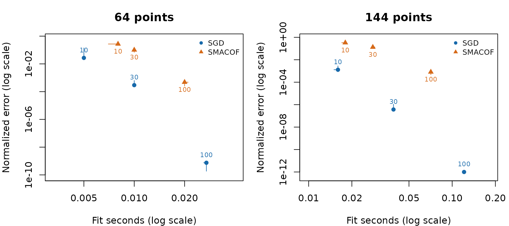
Separate schedules: median normalized error versus median fitting time; bars show the interquartile ranges over five starts. Labels are pass/iteration allowances.

64 points

Method	Raw stress	Normalized error	Fit seconds	Passes/iterations	Termination
Generating reference	0.000e+00	0.000e+00	NA	NA	Reference only
Classical MDS	2.474e-27	4.736e-16	0.002	NA	Spectral reference
SGD	1.843e-12	1.293e-08	0.027	100	iteration_limit
SMACOF	7.103e-04	2.537e-04	0.020	100	iteration_limit

Fixed seed 1, allowance 100. Gray: generating reference; blue: SGD; orange: SMACOF. The table above reports the exact displayed fits. Alignment preserves scale.

Gaussian cloud 64 points; Ambient Euclidean targets. Gray: reference; blue: SGD; orange: SMACOF. Rigid alignment only.

144 points

Method	Raw stress	Normalized error	Fit seconds	Passes/iterations	Termination
Generating reference	0.000e+00	0.000e+00	NA	NA	Reference only
Classical MDS	5.115e-26	9.146e-16	0.002	NA	Spectral reference
SGD	3.615e-26	7.689e-16	0.121	100	iteration_limit
SMACOF	7.153e-01	3.420e-03	0.071	100	iteration_limit

Fixed seed 1, allowance 100. Gray: generating reference; blue: SGD; orange: SMACOF. The table above reports the exact displayed fits. Alignment preserves scale.

Gaussian cloud 144 points; Ambient Euclidean targets. Gray: reference; blue: SGD; orange: SMACOF. Rigid alignment only.

Plane: Ambient Euclidean

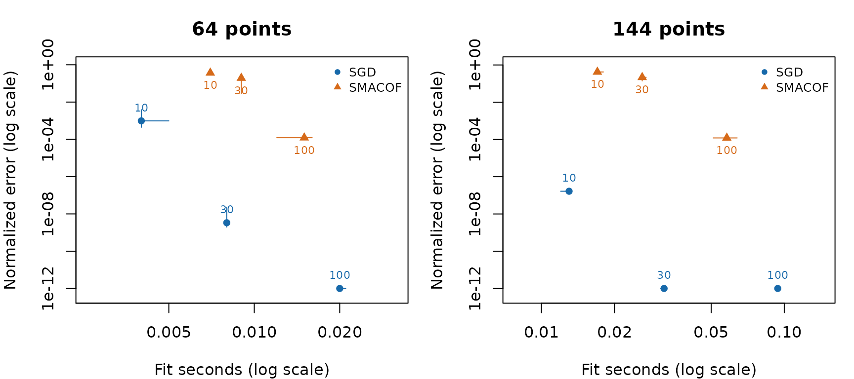
Separate schedules: median normalized error versus median fitting time; bars show the interquartile ranges over five starts. Labels are pass/iteration allowances.

64 points

Method	Raw stress	Normalized error	Fit seconds	Passes/iterations	Termination
Generating reference	1.613e-29	6.779e-17	NA	NA	Reference only
Classical MDS	1.008e-26	1.695e-15	0.001	NA	Spectral reference
SGD	1.165e-28	1.822e-16	0.021	100	iteration_limit
SMACOF	5.238e-05	1.222e-04	0.015	75	stress_tolerance

Fixed seed 1, allowance 100. Gray: generating reference; blue: SGD; orange: SMACOF. The table above reports the exact displayed fits. Alignment preserves scale.

144 points

Method	Raw stress	Normalized error	Fit seconds	Passes/iterations	Termination
Generating reference	3.706e-29	4.763e-17	NA	NA	Reference only
Classical MDS	9.170e-27	7.492e-16	0.002	NA	Spectral reference
SGD	2.585e-28	1.258e-16	0.093	100	iteration_limit
SMACOF	2.217e-04	1.165e-04	0.036	53	stress_tolerance

Fixed seed 1, allowance 100. Gray: generating reference; blue: SGD; orange: SMACOF. The table above reports the exact displayed fits. Alignment preserves scale.

Paraboloid: Ambient Euclidean

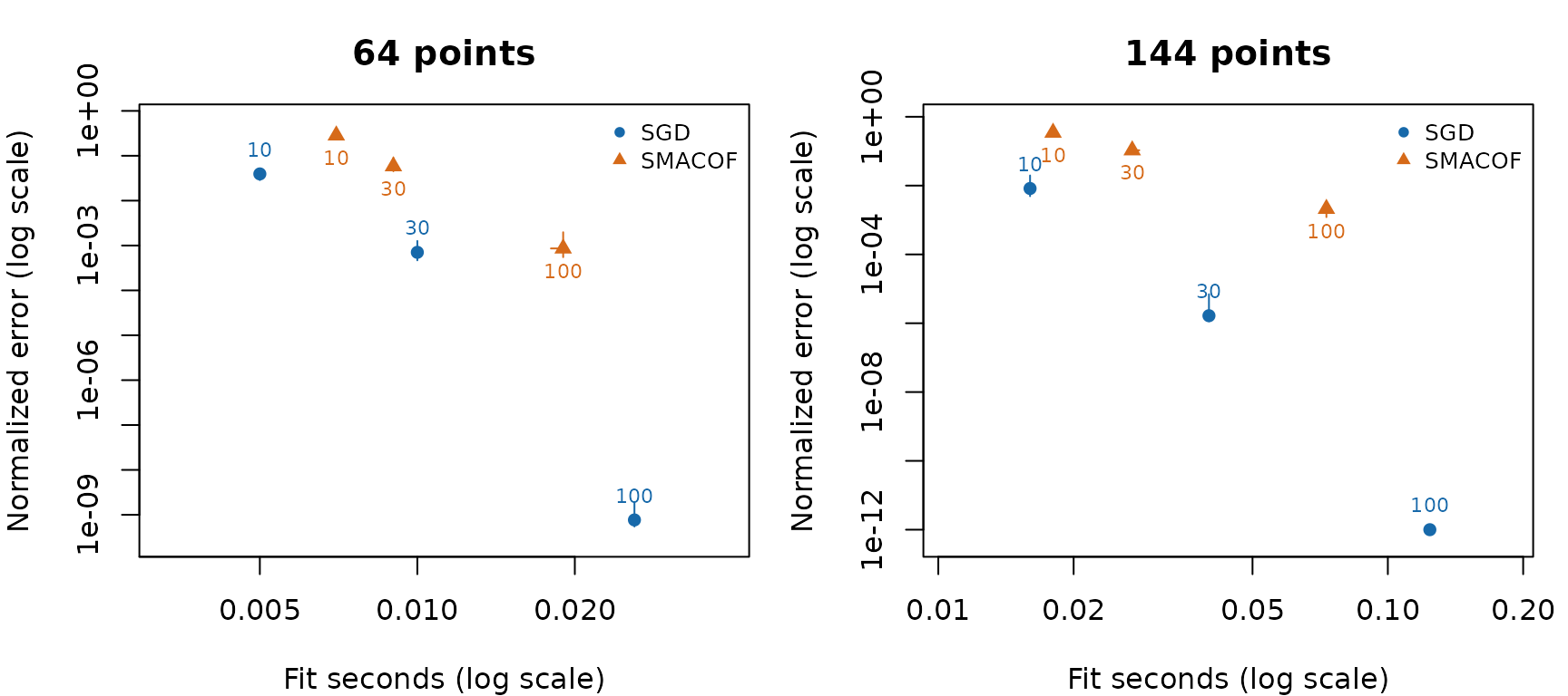
Separate schedules: median normalized error versus median fitting time; bars show the interquartile ranges over five starts. Labels are pass/iteration allowances.

64 points

Method	Raw stress	Normalized error	Fit seconds	Passes/iterations	Termination
Generating reference	0.000e+00	0.000e+00	NA	NA	Reference only
Classical MDS	3.208e-27	8.693e-16	0.000	NA	Spectral reference
SGD	2.392e-16	2.374e-10	0.026	100	iteration_limit
SMACOF	3.144e-03	8.607e-04	0.018	100	iteration_limit

Fixed seed 1, allowance 100. Gray: generating reference; blue: SGD; orange: SMACOF. The table above reports the exact displayed fits. Alignment preserves scale.

Paraboloid 64 points; Ambient Euclidean targets. Gray: reference; blue: SGD; orange: SMACOF. Rigid alignment only.

144 points

Method	Raw stress	Normalized error	Fit seconds	Passes/iterations	Termination
Generating reference	0.000e+00	0.000e+00	NA	NA	Reference only
Classical MDS	2.416e-26	1.111e-15	0.002	NA	Spectral reference
SGD	1.086e-26	7.450e-16	0.126	100	iteration_limit
SMACOF	6.630e-01	5.821e-03	0.074	100	iteration_limit

Fixed seed 1, allowance 100. Gray: generating reference; blue: SGD; orange: SMACOF. The table above reports the exact displayed fits. Alignment preserves scale.

Paraboloid 144 points; Ambient Euclidean targets. Gray: reference; blue: SGD; orange: SMACOF. Rigid alignment only.

Saddle: Ambient Euclidean

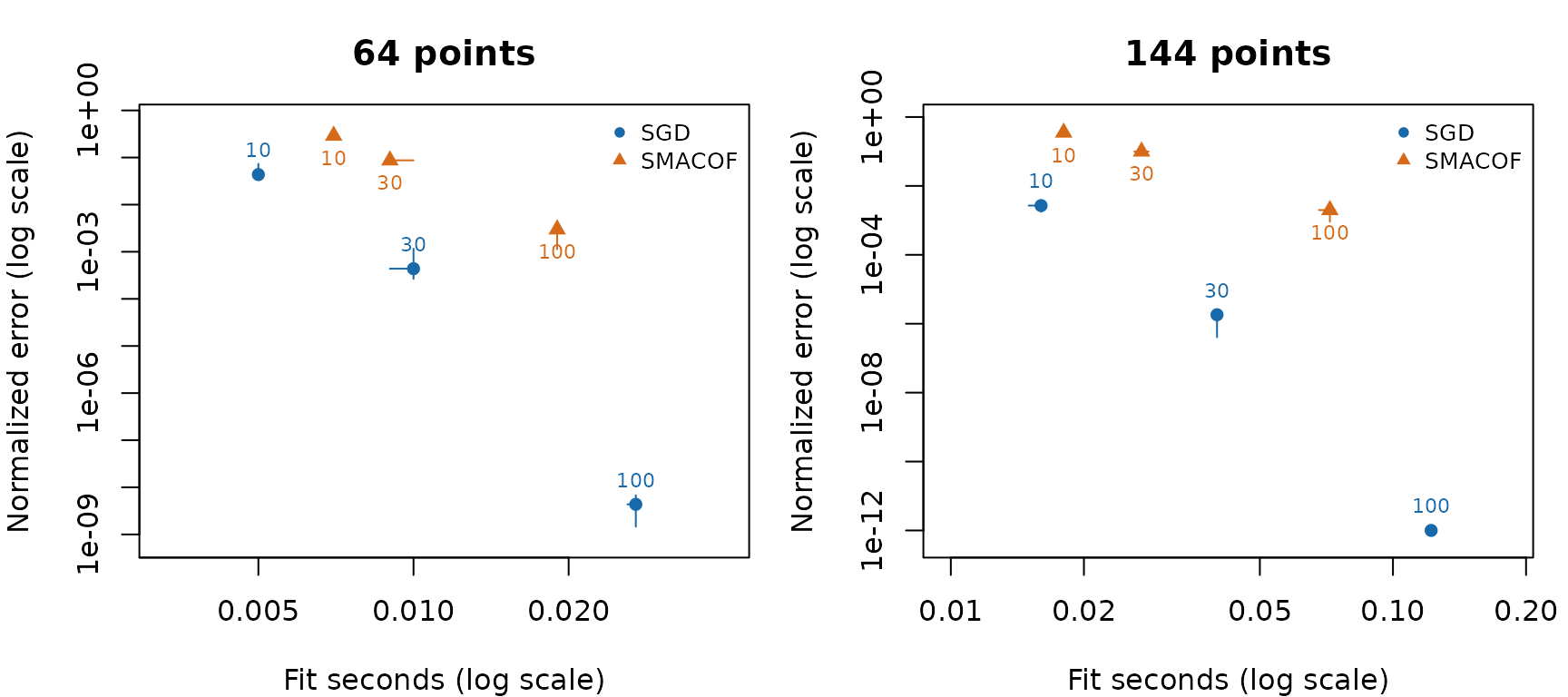
Separate schedules: median normalized error versus median fitting time; bars show the interquartile ranges over five starts. Labels are pass/iteration allowances.

64 points

Method	Raw stress	Normalized error	Fit seconds	Passes/iterations	Termination
Generating reference	4.745e-30	3.344e-17	NA	NA	Reference only
Classical MDS	2.021e-27	6.901e-16	0.001	NA	Spectral reference
SGD	9.097e-15	1.464e-09	0.027	100	iteration_limit
SMACOF	3.787e-02	2.987e-03	0.019	100	iteration_limit

Fixed seed 1, allowance 100. Gray: generating reference; blue: SGD; orange: SMACOF. The table above reports the exact displayed fits. Alignment preserves scale.

Saddle 64 points; Ambient Euclidean targets. Gray: reference; blue: SGD; orange: SMACOF. Rigid alignment only.

144 points

Method	Raw stress	Normalized error	Fit seconds	Passes/iterations	Termination
Generating reference	2.523e-29	3.591e-17	NA	NA	Reference only
Classical MDS	1.016e-26	7.207e-16	0.003	NA	Spectral reference
SGD	1.092e-26	7.472e-16	0.122	100	iteration_limit
SMACOF	1.161e-03	2.436e-04	0.074	95	stress_tolerance

Fixed seed 1, allowance 100. Gray: generating reference; blue: SGD; orange: SMACOF. The table above reports the exact displayed fits. Alignment preserves scale.

Saddle 144 points; Ambient Euclidean targets. Gray: reference; blue: SGD; orange: SMACOF. Rigid alignment only.

Paraboloid: Local graph paths

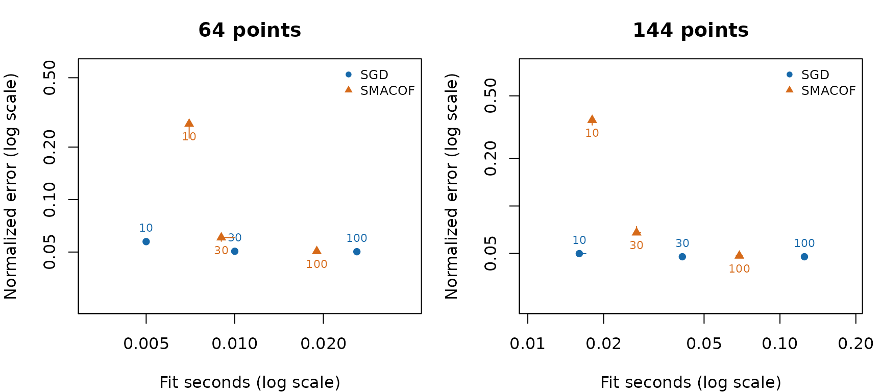
Separate schedules: median normalized error versus median fitting time; bars show the interquartile ranges over five starts. Labels are pass/iteration allowances.

64 points

Method	Raw stress	Normalized error	Fit seconds	Passes/iterations	Termination
Generating reference	1.773e+02	1.732e-01	NA	NA	Reference only
Classical MDS	1.650e+01	5.283e-02	0.001	NA	Spectral reference
SGD	1.491e+01	5.023e-02	0.026	100	iteration_limit
SMACOF	1.506e+01	5.049e-02	0.019	100	iteration_limit

Fixed seed 1, allowance 100. Gray: generating reference; blue: SGD; orange: SMACOF. The table above reports the exact displayed fits. Alignment preserves scale.

Paraboloid 64 points; Local graph paths targets. Gray: reference; blue: SGD; orange: SMACOF. Rigid alignment only.

144 points

Method	Raw stress	Normalized error	Fit seconds	Passes/iterations	Termination
Generating reference	7.825e+02	1.698e-01	NA	NA	Reference only
Classical MDS	6.948e+01	5.059e-02	0.006	NA	Spectral reference
SGD	6.152e+01	4.761e-02	0.125	100	iteration_limit
SMACOF	7.396e+01	5.220e-02	0.072	100	iteration_limit

Fixed seed 1, allowance 100. Gray: generating reference; blue: SGD; orange: SMACOF. The table above reports the exact displayed fits. Alignment preserves scale.

Paraboloid 144 points; Local graph paths targets. Gray: reference; blue: SGD; orange: SMACOF. Rigid alignment only.

Saddle: Local graph paths

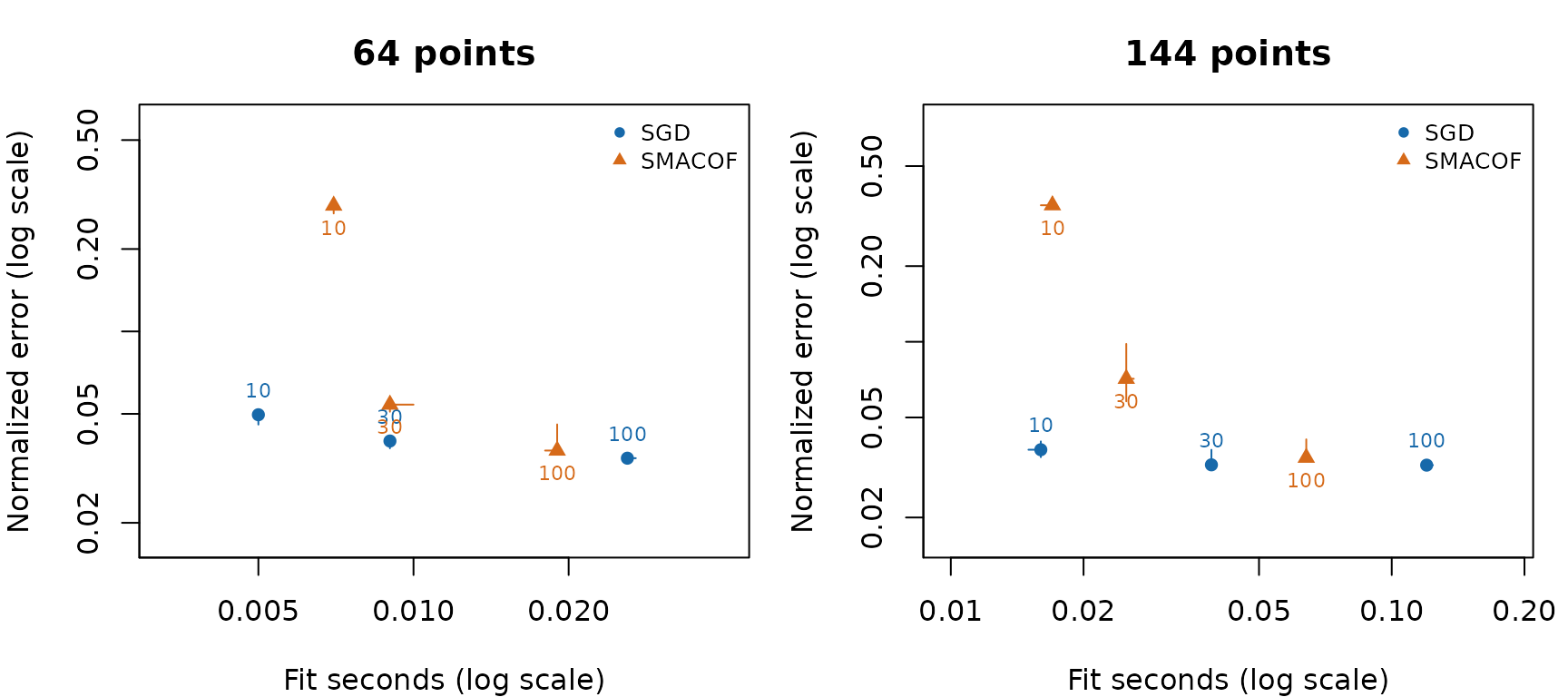
Separate schedules: median normalized error versus median fitting time; bars show the interquartile ranges over five starts. Labels are pass/iteration allowances.

64 points

Method	Raw stress	Normalized error	Fit seconds	Passes/iterations	Termination
Generating reference	7.164e+01	1.175e-01	NA	NA	Reference only
Classical MDS	9.073e+00	4.183e-02	0.001	NA	Spectral reference
SGD	6.154e+00	3.445e-02	0.027	100	iteration_limit
SMACOF	1.105e+01	4.615e-02	0.019	100	iteration_limit

Fixed seed 1, allowance 100. Gray: generating reference; blue: SGD; orange: SMACOF. The table above reports the exact displayed fits. Alignment preserves scale.

Surface-shape alignment

The gray reference stays fixed. The blue and orange layouts are moved to match surface shape rather than vertex labels. Choose SGD, SMACOF, or both.

Backend	Subdivisions per edge	Surface RMS before	Surface RMS after
SGD	6	0.3528	0.1588
SGD	9	0.3524	0.1579
SMACOF	6	0.2916	0.2378
SMACOF	9	0.2911	0.2369

Saddle 64 points. Surface-shape alignment; scale unchanged. Gray: reference; blue: SGD; orange: SMACOF.

144 points

Method	Raw stress	Normalized error	Fit seconds	Passes/iterations	Termination
Generating reference	3.116e+02	1.143e-01	NA	NA	Reference only
Classical MDS	3.776e+01	3.979e-02	0.005	NA	Spectral reference
SGD	2.491e+01	3.232e-02	0.120	100	iteration_limit
SMACOF	3.993e+01	4.092e-02	0.063	100	iteration_limit

Fixed seed 1, allowance 100. Gray: generating reference; blue: SGD; orange: SMACOF. The table above reports the exact displayed fits. Alignment preserves scale.

Surface-shape alignment

The gray reference stays fixed. The blue and orange layouts are moved to match surface shape rather than vertex labels. Choose SGD, SMACOF, or both.

Backend	Subdivisions per edge	Surface RMS before	Surface RMS after
SGD	6	0.3708	0.1511
SGD	9	0.3706	0.1506
SMACOF	6	0.1742	0.1737
SMACOF	9	0.1738	0.1734

Saddle 144 points. Surface-shape alignment; scale unchanged. Gray: reference; blue: SGD; orange: SMACOF.

Spatial helix graph: Local graph paths

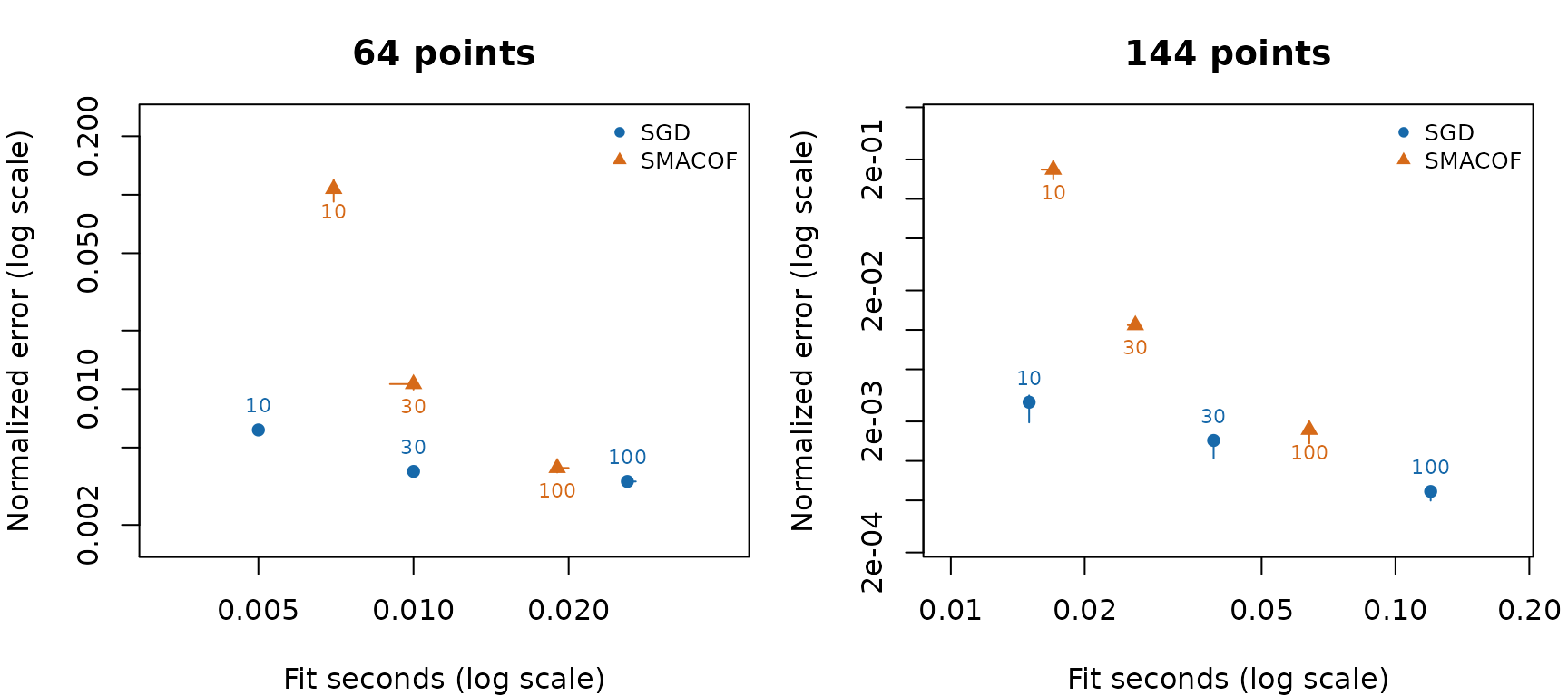
Separate schedules: median normalized error versus median fitting time; bars show the interquartile ranges over five starts. Labels are pass/iteration allowances.

64 points

Method	Raw stress	Normalized error	Fit seconds	Passes/iterations	Termination
Generating reference	1.084e+04	5.825e-01	NA	NA	Reference only
Classical MDS	3.686e+00	1.074e-02	0.001	NA	Spectral reference
SGD	3.605e-01	3.359e-03	0.027	100	iteration_limit
SMACOF	4.930e-01	3.929e-03	0.020	100	iteration_limit

Fixed seed 1, allowance 100. Gray: generating reference; blue: SGD; orange: SMACOF. The table above reports the exact displayed fits. Alignment preserves scale.

Spatial helix graph 64 points; Local graph paths targets. Gray: reference; blue: SGD; orange: SMACOF. Rigid alignment only.

144 points

Method	Raw stress	Normalized error	Fit seconds	Passes/iterations	Termination
Generating reference	5.935e+04	5.930e-01	NA	NA	Reference only
Classical MDS	4.922e-01	1.708e-03	0.003	NA	Spectral reference
SGD	6.197e-02	6.059e-04	0.119	100	iteration_limit
SMACOF	9.666e-01	2.393e-03	0.063	100	iteration_limit

Fixed seed 1, allowance 100. Gray: generating reference; blue: SGD; orange: SMACOF. The table above reports the exact displayed fits. Alignment preserves scale.

Spatial helix graph 144 points; Local graph paths targets. Gray: reference; blue: SGD; orange: SMACOF. Rigid alignment only.

Surface alignment uses symmetric iterative closest-point matching on the triangulated surfaces. Each triangle is sampled at the centers of nine equal-area subtriangles; samples are weighted by triangle area. The search starts from the vertex-aligned fit at 24 rotations about the reference’s vertical axis, with and without a vertical reflection. Each of the 48 starts allows 80 updates, stopping when the change in mean squared surface distance is at most one billionth of its initial value. Updates can rotate about any axis. The lowest sampled error is selected, retaining the initial alignment if none improves it. This is a local search, not a guarantee of the globally best surface match.

The tables evaluate the result on denser samples: 36 and 81 subtriangles per triangle. Surface RMS is the square root of the mean squared nearest-sample distance, averaged in both directions and weighted by surface area. It is in coordinate units; smaller values indicate closer surfaces. It is an approximation to surface distance, not vertex error or MDS stress. The mesh, its boundary and the underlying fitted coordinates are unchanged.

The effect of stress weighting

Uniform stress measures squared errors in distance units. The paper’s weighting instead minimizes squared relative errors:

$$S_{\mathrm{relative}}(Z) = \sum_{i<j}\frac{(\lVert z_i-z_j\rVert-d_{ij})^2}{d_{ij}^2}.$$

For example, an error of 0.2 on a target distance of 1 counts as much as an error of 2 on a target distance of 10. Thus shorter distances receive more influence than under uniform weighting. This changes the objective for both optimizers; it is separate from the edge lengths used to compute graph shortest paths.

Select the same weighting for either backend:

sgd <- metric.mds(prepared = prepared, dim = 3, init = start,
                 backend = "sgd", pair.weights = "inverse_squared",
                 max.iter = 100, diagnostics = FALSE)
smacof <- metric.mds(prepared = prepared, dim = 3, init = start,
                    backend = "smacof", pair.weights = "inverse_squared",
                    max.iter = 100, eps = 1e-8, diagnostics = FALSE)

Set pair.weights = "uniform" to use the original objective. Inverse-squared weighting requires positive distances between distinct vertices; zero distances are rejected rather than replaced by a small constant. The learning-rate schedule stays the same as above, in RMS-normalized distance units. These fits use the paper’s weighting, with grip’s documented schedule and initialization.

This separate 60-fit experiment compares the saddle, paraboloid, and spatial helix graphs with 64 vertices each. Each backend and weighting receives the same five random starting shapes, seeds 1–5, with one start per fit and an allowance of 100 passes or iterations. The wrapper fits the initial and final coordinate scale to the selected objective. The allowance, SGD controls, and SMACOF tolerance match the original comparison. Each worker has 30 seconds; the whole experiment has 600 seconds. Failed fits remain in the results.

Every returned layout is scored under both definitions: uniform normalized error and root-mean-square relative error. Compare rows within the same error column. The two columns measure different goals; their magnitudes do not select a universally better weighting. Reported scores use the returned coordinates without fitting another scale for the other objective.

The run returned coordinates for 60 of 60 fits. As above, a returned fit does not imply convergence. Tables give medians across all five starts and then the scores of the exact displayed runs. The figures use the preselected seed 1. All four layouts and the gray generating reference share the same camera and scale; the saddle uses the surface-shape alignment described above for all four backend/weighting combinations. The other examples use vertex-based Procrustes alignment. Neither alignment resizes or deforms the layouts.

In this run, inverse-squared weighting lowered median relative error in 6 of 6 graph–backend comparisons, while increasing median uniform error in 6. The figures show how that change in priorities alters each layout.

Saddle: uniform versus inverse-squared weights

Medians across five starting shapes:

Backend	Weighting	Returned	Attempted	Uniform error	Relative error	Fit seconds
SGD	Uniform	5	5	0.0344	0.0435	0.027
SMACOF	Uniform	5	5	0.0367	0.0458	0.018
SMACOF	Inverse-squared	5	5	0.0422	0.0442	0.019
SGD	Inverse-squared	5	5	0.0383	0.0401	0.027

Displayed runs (seed 1):

Backend	Weighting	Uniform error	Relative error	Fit seconds	Termination	Status
SGD	Uniform	0.0344	0.0435	0.027	iteration_limit	ok
SGD	Inverse-squared	0.0382	0.0401	0.027	iteration_limit	ok
SMACOF	Uniform	0.0462	0.0536	0.018	iteration_limit	ok
SMACOF	Inverse-squared	0.0385	0.0403	0.018	iteration_limit	ok

Saddle 64 points. Surface-shape alignment; scale unchanged. Gray: reference; blue/green: SGD with uniform/inverse-squared weights; orange/purple: SMACOF with uniform/inverse-squared weights.

Paraboloid: uniform versus inverse-squared weights

Medians across five starting shapes:

Backend	Weighting	Returned	Attempted	Uniform error	Relative error	Fit seconds
SGD	Uniform	5	5	0.0502	0.0623	0.027
SMACOF	Uniform	5	5	0.0505	0.0625	0.019
SMACOF	Inverse-squared	5	5	0.0605	0.0529	0.019
SGD	Inverse-squared	5	5	0.0608	0.0529	0.027

Displayed runs (seed 1):

Backend	Weighting	Uniform error	Relative error	Fit seconds	Termination	Status
SGD	Uniform	0.0502	0.0623	0.027	iteration_limit	ok
SGD	Inverse-squared	0.0608	0.0529	0.027	iteration_limit	ok
SMACOF	Uniform	0.0505	0.0625	0.020	iteration_limit	ok
SMACOF	Inverse-squared	0.0605	0.0529	0.020	iteration_limit	ok

Paraboloid 64 vertices. Gray: reference; blue/green: SGD with uniform/inverse-squared weights; orange/purple: SMACOF with uniform/inverse-squared weights. Alignment preserves scale.

Spatial helix graph: uniform versus inverse-squared weights

Medians across five starting shapes:

Backend	Weighting	Returned	Attempted	Uniform error	Relative error	Fit seconds
SGD	Uniform	5	5	0.0033	0.0104	0.027
SMACOF	Uniform	5	5	0.0039	0.0155	0.019
SMACOF	Inverse-squared	5	5	0.0154	0.0125	0.019
SGD	Inverse-squared	5	5	0.0050	0.0085	0.027

Displayed runs (seed 1):

Backend	Weighting	Uniform error	Relative error	Fit seconds	Termination	Status
SGD	Uniform	0.0034	0.0104	0.027	iteration_limit	ok
SGD	Inverse-squared	0.0051	0.0082	0.027	iteration_limit	ok
SMACOF	Uniform	0.0039	0.0171	0.019	iteration_limit	ok
SMACOF	Inverse-squared	0.0161	0.0126	0.019	iteration_limit	ok

Spatial helix graph 64 vertices. Gray: reference; blue/green: SGD with uniform/inverse-squared weights; orange/purple: SMACOF with uniform/inverse-squared weights. Alignment preserves scale.

Sparse SGD for larger graphs

metric.mds(approximation = "sparse") uses representative vertices (pivots) to approximate long-range interactions while retaining graph edges. It implements the sparse SGD method of Zheng et al. (2018), based on Ortmann et al. (2017), with inverse-squared weighting and no all-pairs distance preparation.

See Sparse SGD for larger graphs for usage and a separate comparison of full SGD, sparse SGD with several pivot counts, and weighted GRIP. It includes 3D views, repeated runs, total layout times, measured peak memory, and an independently scored 4,096-vertex saddle.

Reproduce the experiment

Building this vignette runs the small example and displays saved results for the larger comparison. To repeat all 420 fits, install the R packages callr and smacof, then run these commands in the grip source folder:

mkdir -p ../comparison-library
R CMD INSTALL --preclean --library=../comparison-library . > ../comparison-install.log 2>&1
Rscript tools/pkg/build-metric-mds-comparison.R ../fresh-results ../comparison-library ../comparison-install.log

To repeat the separate weighting comparison, add weighting as the final argument and choose another results folder:

Rscript tools/pkg/build-metric-mds-comparison.R ../fresh-weighting-results ../comparison-library ../comparison-install.log weighting

The script saves the timings, fitted coordinates, and any errors in fresh-results, beside the grip source folder. Choose a new results folder for each run. Instructions for recreating the figures are in the reproduction guide.

References

• Zheng, J. X., Pawar, S. and Goodman, D. F. (2018). Graph Drawing by Stochastic Gradient Descent. doi:10.1109/TVCG.2018.2859997.

• Hangan, D., Kobourov, S. and Miller, J. (2026). Bridging Graph Drawing and Dimensionality Reduction with Stochastic Stress Optimization. arXiv:2605.00641.

• Mair, P., Groenen, P. J. F. and de Leeuw, J. (2022). More on Multidimensional Scaling and Unfolding in R: smacof Version 2. Journal of Statistical Software, 102(10). doi:10.18637/jss.v102.i10.