Comparing grip with Alternative Layout Engines • grip

This website-only article complements the installed function guide and synthetic graph examples.

What is compared

grip is no longer just an R implementation of the classical GRIP algorithm. The package now contains:

a quality-first GRIP workflow for ordinary graphs,
weighted geometry-aware sister APIs,
and geodesic scoring and polishing utilities.

That means there are now two different comparison questions:

how the saved grip 0.2.0 results compare with other R layout engines on ordinary unweighted graphs,
how geometry-aware weighted grip methods behave on weighted graphs, where plain topology is not the whole problem.

This article treats those as separate tracks.

library(grip)

Shared scoring idea

score.layout() can score a realized layout from any source. That remains one of the most useful parts of the package, because it lets you compare candidate layouts even when they come from different packages.

score_layout <- function(coords, edges, n,
                         clusters = NULL,
                         edge.crossings = "auto",
                         sample.size.stress = 2000L,
                         sample.size.nonedge = 5000L) {
  score.layout(
    coords = coords,
    edges = edges,
    n = n,
    clusters = clusters,
    sample.size.stress = sample.size.stress,
    sample.size.nonedge = sample.size.nonedge,
    stress.seed = 42L,
    nonedge.seed = 42L,
    edge.crossings = edge.crossings
  )
}

For weighted geometry-aware graphs, the package also provides retained-path diagnostics that answer a different question from sampled chord stress:

Those GKK/LGKK-style tools are advanced public experimental utilities rather than the default onboarding path, and they are used in the second half of this article for the weighted comparison track.

plot_layout <- function(coords,
                        edges,
                        title,
                        vertex.col = "#1F3B73",
                        edge.col = "gray80",
                        cex = 0.55) {
  if (ncol(coords) == 2L) {
    plot(
      coords[, 1], coords[, 2],
      asp = 1,
      pch = 16,
      cex = cex,
      col = vertex.col,
      xlab = "",
      ylab = "",
      axes = FALSE,
      main = title
    )
    if (!is.null(edges) && nrow(edges) > 0) {
      segments(
        coords[edges[, 1], 1], coords[edges[, 1], 2],
        coords[edges[, 2], 1], coords[edges[, 2], 2],
        col = edge.col
      )
    }
  } else {
    plot.layout(
      coords,
      edges,
      projection = "ortho",
      azimuth = 35,
      elevation = 22,
      vertex.col = vertex.col,
      edge.col = edge.col,
      main = title
    )
  }
}

Track 1: external-package comparisons on unweighted graphs

For this track the comparison remains package-to-package:

igraph
graphlayouts
grip

To keep the article lightweight, the cross-package results are precomputed and bundled as an RDS file. The reproduction script is still:

inst/scripts/precompute-vs-alternatives.R

res.path <- system.file(
  "extdata", "vs_alternatives", "benchmark_results.rds",
  package = "grip"
)
if (!nzchar(res.path)) {
  stop(
    "Precomputed benchmark results not found. ",
    "Run inst/scripts/precompute-vs-alternatives.R first."
  )
}
res <- readRDS(res.path)

Provenance of the saved comparison

The external results were generated on 23 August 2026 with grip 0.2.0. They are frozen results, not reruns of the development version serving this page. The provenance record and reproduction script record the settings and timing boundaries. The artifact’s software versions are:

knitr::kable(data.frame(
  Package = names(res$benchmark_metadata$package_versions),
  Version = unname(res$benchmark_metadata$package_versions)
), row.names = FALSE)

Package	Version
grip	0.2.0
igraph	2.3.3
graphlayouts	1.2.5

The karate graph has 34 vertices and 78 edges; the 12 by 12 mesh has 144 vertices and 264 edges. Each table below scores a saved layout with hop-distance stress, scoring seeds 42, 2,000 requested stress pairs, and up to 5,000 sampled nonedges. Exact crossings are enabled for these small graphs. The stress score fits a common scale; it is not the raw stress objective of metric.mds(). Preset/tuned rows are labeled separately from ordinary defaults. Keep the results where another method scores better when interpreting the comparison.

Benchmark 1: Zachary karate club

This is still a useful small-graph sanity check. The graph is small enough that single-scale methods can compete directly.

karate.display <- res$karate$scores[, c(
  "method",
  "sampled.stress",
  "edge.length.cv",
  "edge.crossings",
  "sampled.nonedge.sep.ratio",
  "cluster.separation"
)]

knitr::kable(
  karate.display,
  digits = 4,
  row.names = FALSE,
  caption = "Karate club: saved grip 0.2.0 benchmark; one seeded layout per method."
)

Karate club: saved grip 0.2.0 benchmark; one seeded layout per method.
method	sampled.stress	edge.length.cv	edge.crossings	sampled.nonedge.sep.ratio	cluster.separation
FR (igraph)	0.2477	0.3581	68	0.3670	2.7566
KK (igraph)	0.2102	0.2806	73	0.3021	2.2528
DrL (igraph)	0.3320	0.4680	120	0.2372	1.6584
Stress (graphlayouts)	0.2075	0.2611	78	0.2747	2.2240
grip default	0.2221	0.2941	75	0.2547	2.1364
grip tuned	0.3254	0.2836	124	0.0570	1.7389

k <- res$karate
par(mfrow = c(2, 3), mar = c(1, 1, 3, 1), bg = "white")
plot_layout(k$layouts$fr,            k$edges, "FR (igraph)", cex = 0.6)
plot_layout(k$layouts$kk,            k$edges, "KK (igraph)", cex = 0.6)
plot_layout(k$layouts$drl,           k$edges, "DrL (igraph)", cex = 0.6)
plot_layout(k$layouts$stress,        k$edges, "Stress (graphlayouts)", cex = 0.6)
plot_layout(k$layouts$grip.default,  k$edges, "grip default", cex = 0.6)
plot_layout(k$layouts$grip.tuned,    k$edges, "grip tuned", cex = 0.6)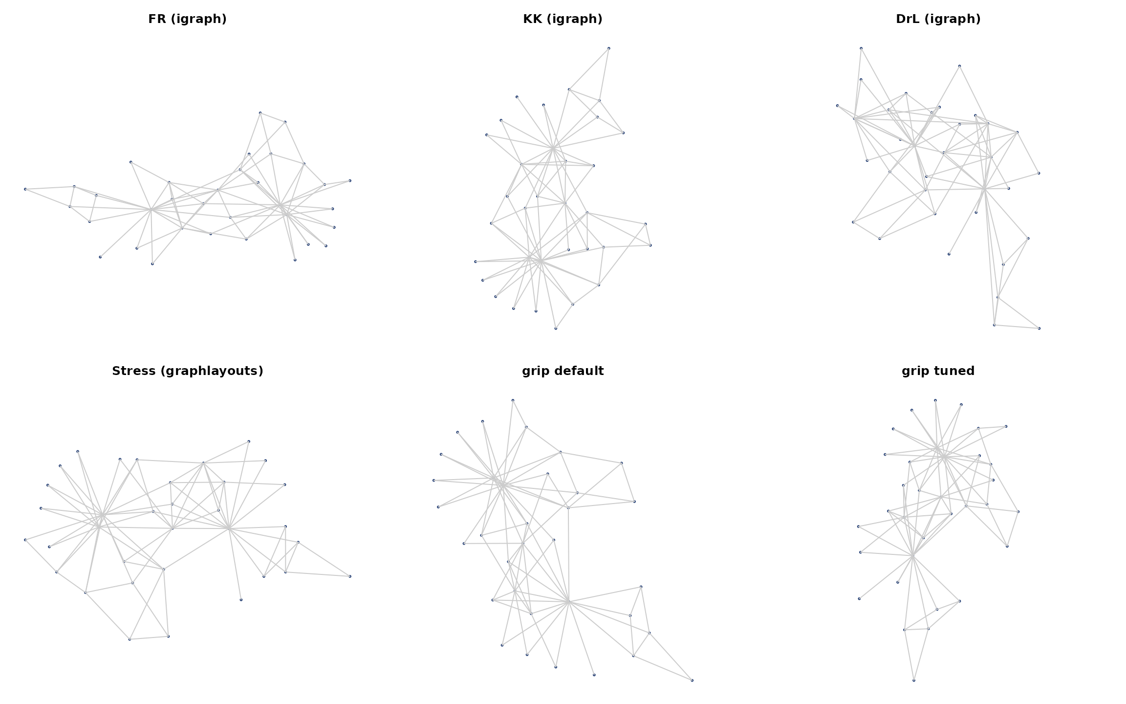

On graphs this small, grip does not have a special structural advantage. That is an honest result and a useful reminder: multiscale methods are not automatically best on every graph.

Benchmark 2: 12x12 mesh

Meshes are a good structured topological benchmark because a strong layout should recover an orderly grid with uniform edge lengths and few or no crossings.

mesh.display <- res$mesh$scores[, c(
  "method",
  "sampled.stress",
  "edge.length.cv",
  "edge.crossings",
  "sampled.nonedge.sep.ratio"
)]

knitr::kable(
  mesh.display,
  digits = 4,
  row.names = FALSE,
  caption = "12x12 mesh: saved grip 0.2.0 benchmark; one seeded layout per method."
)

12x12 mesh: saved grip 0.2.0 benchmark; one seeded layout per method.
method	sampled.stress	edge.length.cv	sampled.nonedge.sep.ratio
FR (igraph)	0.1159	0.1735	0.9731
KK (igraph)	0.1039	0.0135	1.3356
DrL (igraph)	0.1276	0.3580	0.5613
Stress (graphlayouts)	0.1040	0.0138	1.3367
grip default	0.1089	0.0490	1.1589
grip mesh preset	0.1056	0.0497	1.2197

m <- res$mesh
par(mfrow = c(2, 3), mar = c(1, 1, 3, 1), bg = "white")
plot_layout(m$layouts$fr,            m$edges, "FR (igraph)", cex = 0.5)
plot_layout(m$layouts$kk,            m$edges, "KK (igraph)", cex = 0.5)
plot_layout(m$layouts$drl,           m$edges, "DrL (igraph)", cex = 0.5)
plot_layout(m$layouts$stress,        m$edges, "Stress (graphlayouts)", cex = 0.5)
plot_layout(m$layouts$grip.default,  m$edges, "grip default", cex = 0.5)
plot_layout(m$layouts$grip.mesh,     m$edges, "grip mesh preset", cex = 0.5)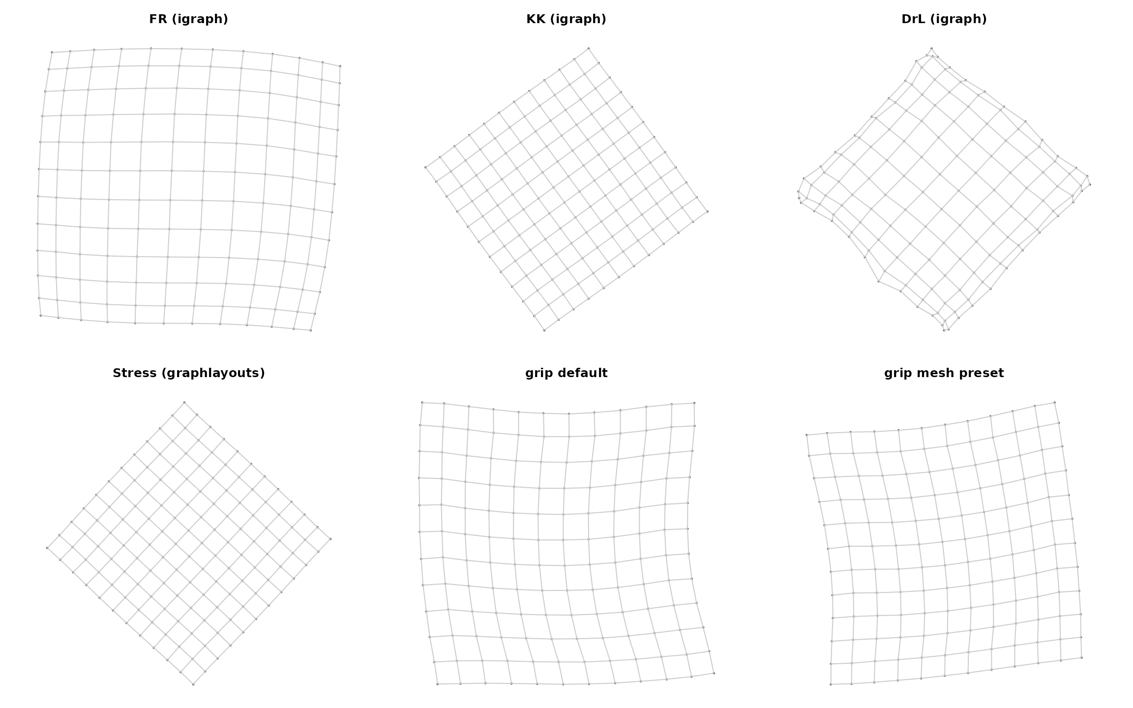

This benchmark shows a different pattern from the karate graph: on a canonical structured family like a mesh, the saved grip 0.2.0 default result shows a clean uncrossed layout. The saved mesh preset result has slightly lower sampled stress. These are particular seeded results, not an estimate of variation across layout seeds. At the same time, stress and KK remain very strong on a regular lattice.

Larger graph: saved HMP timing and quality

The same artifact includes an unweighted symmetric-neighbor graph of HMP microbiome samples: 4,391 vertices and 9,067 edges. PCA-space edge lengths were not supplied to any layout engine. The recorded machine was an Apple M4 Max with 64 GiB memory, macOS/Darwin 25.6.0, and R 4.6.1.

knitr::kable(res$hmp$timing, digits = 3, row.names = FALSE,
  caption = "HMP graph: elapsed seconds for saved grip 0.2.0-era runs.")

HMP graph: elapsed seconds for saved grip 0.2.0-era runs.
method	n.runs	elapsed.sec.median	elapsed.sec.iqr
FR (igraph)	5	0.115	0.001
DrL (igraph)	5	2.840	0.001
Stress (graphlayouts)	5	24.530	0.142
grip default (hop)	5	0.531	0.002

knitr::kable(res$hmp$scores[, c("method", "sampled.stress", "edge.length.cv")],
  digits = 4, row.names = FALSE,
  caption = "HMP graph: hop-distance quality of the first timed layout per method.")

HMP graph: hop-distance quality of the first timed layout per method.
method	sampled.stress	edge.length.cv
FR (igraph)	0.6010	0.7438
DrL (igraph)	0.5122	2.5957
Stress (graphlayouts)	0.1640	0.3587
grip default (hop)	0.2286	0.3464

The five timing repeats reset seed 1 before each layout call. Their medians and interquartile ranges measure timing variation for that seeded setup, not variation across independent stochastic layouts. Timing includes only the layout call; graph construction, garbage collection, and scoring are excluded. Scores use the first repeat, seeds 42, 2,000 stress pairs, and up to 5,000 nonedges; exact crossings are disabled for this graph. These hardware-specific times and single-seed quality results do not establish general speed or accuracy rankings.

What the unweighted track tells us

The saved external-package benchmark has a limited scope:

it compares engines on ordinary unweighted graphs,
it uses a shared scoring function on the same graph for each comparison,
but it does not answer the geometry-aware weighted-layout question.

That second question needs a different benchmark track.

Track 2: geometry-aware comparisons on weighted graphs

For weighted graphs with meaningful edge lengths, a pure topology-only comparison is no longer enough. The weighted track in grip is built around:

grip(metric = "edge_length")
optional experimental LGKK-based refinement
and full geodesic-KK scoring.

The small example below is built and scored live in the vignette. It uses a plain mesh topology whose edge lengths are induced by a curved saddle surface.

weighted.mesh <- mesh.surface.graph(
  5, 5,
  surface = "saddle",
  amplitude = 0.8
)

coords.combinatorial <- grip(
  weighted.mesh$edges,
  n = weighted.mesh$n,
  dim = 3,
  preset = "mesh",
  seed = 1
)

coords.weighted <- grip(metric = "edge_length",
  weighted.mesh$edges,
  n = weighted.mesh$n,
  edge_weights = weighted.mesh$edge_weights,
  dim = 3,
  preset = "mesh",
  seed = 1
)

coords.weighted.lgkk <- grip(metric = "edge_length",
  weighted.mesh$edges,
  n = weighted.mesh$n,
  edge_weights = weighted.mesh$edge_weights,
  dim = 3,
  preset = "mesh",
  lgkk_polish_rounds = 6L,
  seed = 1
)

gkk.prepared <- prepare.geodesic.kk(
  weighted.mesh$edges,
  n = weighted.mesh$n,
  edge_weights = weighted.mesh$edge_weights
)

weighted.summary <- do.call(
  rbind,
  list(
    cbind(
      method = "Combinatorial GRIP",
      score.geodesic.kk(
        coords.combinatorial,
        prepared = gkk.prepared
      )[, c(
        "gkk.weighted.rel.rmse",
        "gkk.weighted.rmse",
        "gkk.mean.rel.path.error"
      )]
    ),
    cbind(
      method = "Weighted GRIP",
      score.geodesic.kk(
        coords.weighted,
        prepared = gkk.prepared
      )[, c(
        "gkk.weighted.rel.rmse",
        "gkk.weighted.rmse",
        "gkk.mean.rel.path.error"
      )]
    ),
    cbind(
      method = "Weighted GRIP + LGKK polish",
      score.geodesic.kk(
        coords.weighted.lgkk,
        prepared = gkk.prepared
      )[, c(
        "gkk.weighted.rel.rmse",
        "gkk.weighted.rmse",
        "gkk.mean.rel.path.error"
      )]
    )
  )
)

knitr::kable(
  weighted.summary,
  digits = 4,
  row.names = FALSE,
  caption = "Weighted mesh surface: geodesic-KK comparison metrics."
)

Weighted mesh surface: geodesic-KK comparison metrics.
method	gkk.weighted.rel.rmse	gkk.weighted.rmse	gkk.mean.rel.path.error
Combinatorial GRIP	0.1938	7.1503	0.0978
Weighted GRIP	0.1034	3.7756	0.0538
Weighted GRIP + LGKK polish	0.0030	0.1066	0.0012

par(mfrow = c(2, 2), mar = c(1, 1, 3, 1), bg = "white")
plot_layout(weighted.mesh$coords_surface, weighted.mesh$edges, "Target geometry")
plot_layout(coords.combinatorial, weighted.mesh$edges, "Combinatorial GRIP")
plot_layout(coords.weighted, weighted.mesh$edges, "Weighted GRIP")
plot_layout(coords.weighted.lgkk, weighted.mesh$edges, "Weighted GRIP + LGKK polish")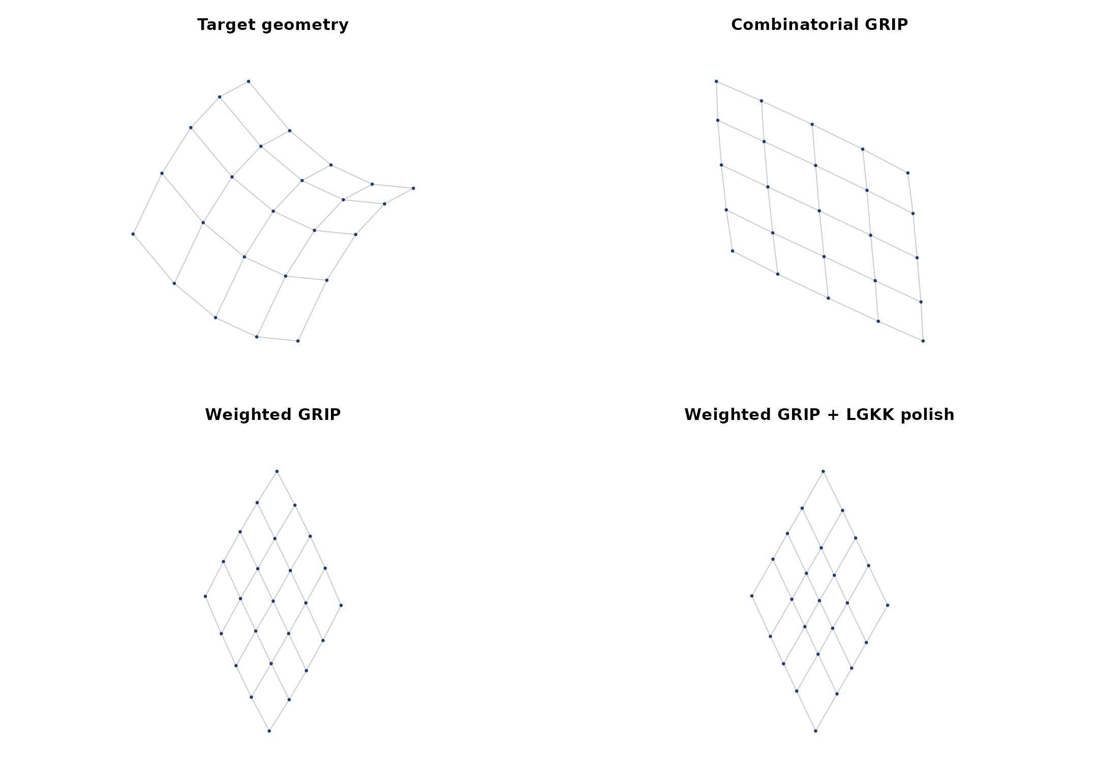

This weighted section is not a package-versus-package benchmark in the old sense. Instead, it answers the more relevant question for modern grip:

what happens when the graph metric matters?

On this example the progression is exactly what the current package design aims for:

combinatorial GRIP gives a topology-respecting layout,
weighted GRIP improves geodesic fidelity,
weighted GRIP plus experimental LGKK polish improves it further.

So what should you compare with what?

For ordinary unweighted graphs:

compare grip with igraph and graphlayouts,
use score.layout() to evaluate all of them on the same graph,
and expect the answer to depend on graph family and graph size.

For weighted geometric graphs:

start with grip(metric = "edge_length"),
use 3D as the primary layout space when the geometry demands it,
and evaluate candidate layouts with geodesic-aware criteria such as score.geodesic.kk().

That is the main conceptual change in the package since the original version of this article was written.

Reproducing the external benchmark bundle

To regenerate the precomputed external-package results in the current working directory:

Sys.setenv(GRIP_VS_ALTERNATIVES_OUTPUT = "benchmark_results.rds")
source(system.file(
  "scripts", "precompute-vs-alternatives.R",
  package = "grip"
))

The weighted section of this article is generated directly inside the vignette, so it reflects the package version used for this website build (0.2.0.9001). It is separate from the frozen external-package results and their timing evidence.

Session info for the bundled external results

res$session_info
#> R version 4.6.1 (2026-06-24)
#> Platform: aarch64-apple-darwin23
#> Running under: macOS Tahoe 26.6.1
#> 
#> Matrix products: default
#> BLAS:   /private/tmp/grip-r-release.FSGPDT/expanded/R-fw.pkg/Payload/R.framework/Versions/4.6/Resources/lib/libRblas.0.dylib 
#> LAPACK: /private/tmp/grip-r-release.FSGPDT/expanded/R-fw.pkg/Payload/R.framework/Versions/4.6/Resources/lib/libRlapack.dylib;  LAPACK version 3.12.1
#> 
#> locale:
#> [1] C.UTF-8/C.UTF-8/C.UTF-8/C/C.UTF-8/C.UTF-8
#> 
#> time zone: America/New_York
#> tzcode source: internal
#> 
#> attached base packages:
#> [1] stats     graphics  grDevices utils     datasets  methods   base     
#> 
#> other attached packages:
#> [1] graphlayouts_1.2.5 igraph_2.3.3       grip_0.2.0        
#> 
#> loaded via a namespace (and not attached):
#>  [1] compiler_4.6.1  magrittr_2.0.5  R6_2.6.1        rprojroot_2.1.1
#>  [5] cli_3.6.6       tools_4.6.1     Rcpp_1.1.2      desc_1.4.3     
#>  [9] pkgload_1.5.3   pkgbuild_1.4.8  lifecycle_1.0.5 pkgconfig_2.0.3
#> [13] rlang_1.3.0