Weighted Graph Layouts with grip • grip

Why weighted layouts deserve their own vignette

Classical GRIP is fundamentally combinatorial: it sees graph topology through hop-count neighborhoods. The unified grip() interface can instead make positive edge lengths a first-class geometric signal throughout the multiscale hierarchy:

grip(metric = "hop") selects the topology-first engine,
grip(metric = "edge_length") selects the edge-length-metric engine,
trace.grip() accepts the same metric choice, and
build.weighted.misf() exposes weighted hierarchy construction directly.

The package decision rule is:

use grip(metric = "hop") for ordinary unweighted or topology-first graphs,
use grip(metric = "edge_length") when edge lengths carry geometry you want to preserve,
add GKK/LGKK only after you already have weighted candidate layouts and need advanced experimental geodesic-aware scoring or polish.

library(grip)

plot.layout.triptych <- function(coords.list,
                                 edges,
                                 titles,
                                 projection = NULL,
                                 vertex.cols = rep("black", length(coords.list)),
                                 edge.col = "gray82") {
  op <- par(
    mfrow = c(1, length(coords.list)),
    mar = c(1.2, 1.2, 3, 1.2),
    bg = "white"
  )
  on.exit(par(op), add = TRUE)

  for (i in seq_along(coords.list)) {
    plot.layout(
      coords.list[[i]], edges,
      projection = projection,
      main = titles[[i]],
      vertex.col = vertex.cols[[i]],
      edge.col = edge.col
    )
  }
}

A first weighted surface example

The helper below creates a plain mesh topology whose edge lengths are induced by a curved 3D surface. The topology stays simple, but the intended metric is no longer the flat grid metric.

surface.mesh <- mesh.surface.graph(
  5, 5,
  surface = "saddle",
  amplitude = 0.9
)

coords.unweighted <- grip(
  surface.mesh$edges,
  n = surface.mesh$n,
  dim = 3,
  preset = "mesh",
  seed = 1
)

coords.weighted <- grip(metric = "edge_length",
  surface.mesh$edges,
  n = surface.mesh$n,
  edge_weights = surface.mesh$edge_weights,
  dim = 3,
  preset = "mesh",
  seed = 1
)

gkk.prepared <- prepare.geodesic.kk(
  surface.mesh$edges,
  n = surface.mesh$n,
  edge_weights = surface.mesh$edge_weights
)

surface.summary <- do.call(
  rbind,
  list(
    cbind(
      method = "Combinatorial GRIP",
      score.geodesic.kk(
        coords.unweighted,
        prepared = gkk.prepared
      )[, c(
        "gkk.weighted.rmse",
        "gkk.mean.abs.path.error",
        "gkk.mean.rel.path.error"
      )]
    ),
    cbind(
      method = "Weighted GRIP",
      score.geodesic.kk(
        coords.weighted,
        prepared = gkk.prepared
      )[, c(
        "gkk.weighted.rmse",
        "gkk.mean.abs.path.error",
        "gkk.mean.rel.path.error"
      )]
    )
  )
)

knitr::kable(surface.summary, digits = 3)

method	gkk.weighted.rmse	gkk.mean.abs.path.error	gkk.mean.rel.path.error
Combinatorial GRIP	7.946	7.394	0.109
Weighted GRIP	4.057	3.911	0.058

plot.layout.triptych(
  list(
    surface.mesh$coords_surface,
    coords.unweighted,
    coords.weighted
  ),
  edges = surface.mesh$edges,
  titles = c("Reference geometry", "Combinatorial GRIP", "Weighted GRIP"),
  projection = "ortho",
  vertex.cols = c("#666666", "black", "#1F3B73")
)

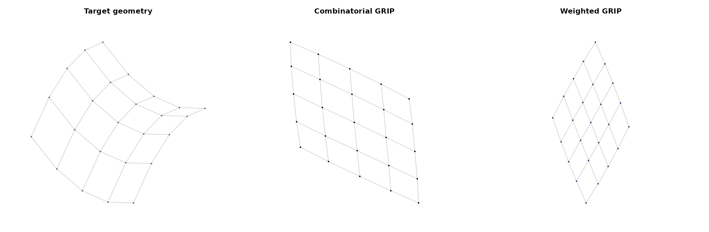
Here the hop fit omits lengths, while the edge-length fit receives them; this changes both the metric and adjacent-edge targets. Topology, vertex order, dimension, preset, and seed are fixed. Both are scored with the same weighted preparation and default scale policy. The reported errors compare lengths accumulated along retained graph paths, not direct recovery of the reference coordinates. This single example is illustrative; see the synthetic-family vignette for a comparison that supplies the same lengths to both fit modes.

2D versus 3D on the same weighted graph

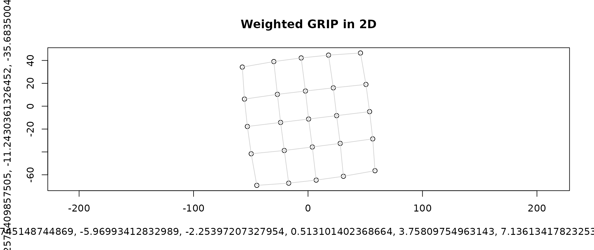
For many weighted geometric families, 3D is the more informative target space. The graph metric can be difficult or impossible to represent faithfully in 2D without substantial distortion.

coords.weighted.2d <- grip(metric = "edge_length",
  surface.mesh$edges,
  n = surface.mesh$n,
  edge_weights = surface.mesh$edge_weights,
  dim = 2,
  preset = "mesh",
  seed = 2
)

coords.weighted.3d <- grip(metric = "edge_length",
  surface.mesh$edges,
  n = surface.mesh$n,
  edge_weights = surface.mesh$edge_weights,
  dim = 3,
  preset = "mesh",
  seed = 2
)

dim.summary <- do.call(
  rbind,
  list(
    cbind(
      dim = "2D",
      score.geodesic.kk(
        coords.weighted.2d,
        prepared = gkk.prepared
      )[, c(
        "gkk.weighted.rmse",
        "gkk.mean.abs.path.error",
        "gkk.mean.rel.path.error"
      )]
    ),
    cbind(
      dim = "3D",
      score.geodesic.kk(
        coords.weighted.3d,
        prepared = gkk.prepared
      )[, c(
        "gkk.weighted.rmse",
        "gkk.mean.abs.path.error",
        "gkk.mean.rel.path.error"
      )]
    )
  )
)

knitr::kable(dim.summary, digits = 3)

dim	gkk.weighted.rmse	gkk.mean.abs.path.error	gkk.mean.rel.path.error
2D	4.060	3.911	0.058
3D	4.056	3.911	0.058

op <- par(mfrow = c(1, 2), mar = c(1.2, 1.2, 3, 1.2), bg = "white")
on.exit(par(op), add = TRUE)

plot.layout(
  coords.weighted.2d,
  surface.mesh$edges,
  main = "Weighted GRIP in 2D",
  vertex.col = "black",
  edge.col = "gray82"
)


plot.layout(
  coords.weighted.3d,
  surface.mesh$edges,
  projection = "ortho",
  main = "Weighted GRIP in 3D",
  vertex.col = "#1F3B73",
  edge.col = "gray82"
)

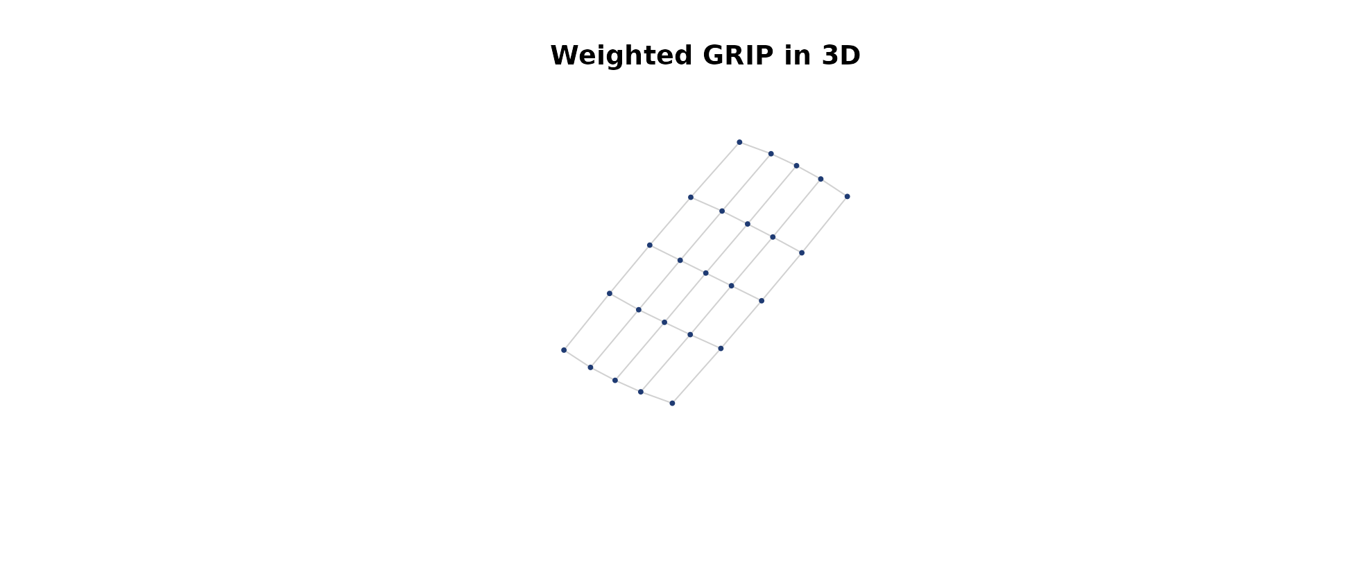
Choose the fitting dimension for the graph and the intended use. This surface has a 3D reference; a 2D drawing remains useful for display, but changes the constraints on the fitted geometry.

Weighted presets

The weighted API keeps explicit presets tuned for the major weighted-family classes currently shipped with the package.

Family class	Good weighted preset	Typical use
Lifted mesh surfaces	`preset = "mesh"`	Rectangular weighted surfaces
Cylindrical grids	`preset = "cylinder"`	Open wrapped surfaces
Toroidal grids	`preset = "torus"`	Closed wrapped surfaces
Near-spherical surfaces	`preset = "sphere"`	Closed surface families
Irregular manifolds and porous families	`preset = "irregular"`	Non-lattice weighted manifolds
Intrinsic weighted trees	`preset = "tree"`	Edge-length-driven tree geometry
Recursive carpet-like lattices	`preset = "carpet"`	Recursive hole-rich weighted grids

These presets are starting points, not declarations that the graph belongs to a single correct family.

Intrinsic weighted trees

Weighted families do not need to come from ambient surfaces. They can also be intrinsically weighted. The example below keeps the topology of a binary tree but assigns edge lengths by depth and branch position.

tree.graph <- kary.tree.weighted.graph(
  k = 2,
  depth = 4,
  depth_rule = "geometric",
  depth_decay = 0.82,
  branch_rule = "linear",
  branch_spread = 0.25
)

tree.coords <- grip(metric = "edge_length",
  tree.graph$edges,
  n = tree.graph$n,
  edge_weights = tree.graph$edge_weights,
  dim = 2,
  preset = "tree",
  seed = 3
)

knitr::kable(
  head(tree.graph$edge_table[, c(
    "parent",
    "child",
    "child_depth",
    "branch_index",
    "edge_weight"
  )]),
  digits = 3
)

parent	child	child_depth	branch_index	edge_weight
1	2	1	1	1.411
1	3	1	2	1.814
2	4	2	1	1.157
2	5	2	2	1.487
3	6	2	1	1.157
3	7	2	2	1.487

plot.layout(
  tree.coords,
  tree.graph$edges,
  main = "Intrinsic weighted tree",
  vertex.col = "#1F3B73",
  edge.col = "gray80",
  pch = 16,
  cex = 0.55
)

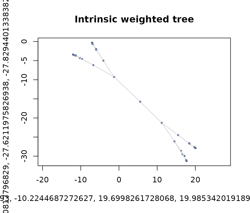
This kind of example is useful because the geometry lives in the edge lengths themselves rather than in a chosen 3D embedding.

Trace and advanced geodesic hooks

The weighted API also supports:

trace.grip(metric = "edge_length") for traced weighted solves,
prepare.geodesic.kk() / score.geodesic.kk() for full GKK evaluation,
prepare.landmark.geodesic.kk() / score.landmark.geodesic.kk() for sparse LGKK evaluation,
lgkk_polish_rounds for post-layout landmark geodesic KK refinement,
lgkk_multiscale_rounds and the stage-specific LGKK controls for in-core multiscale refinement.

These GKK/LGKK tools are public, but they are not the default entry path. For most weighted problems, start with grip(metric = "edge_length") and use the geodesic tools only when you need a stronger metric comparison or an experimental polish step.

Here is the smallest traced weighted example pattern:

surface.trace <- trace.grip(metric = "edge_length",
  surface.mesh$edges,
  n = surface.mesh$n,
  edge_weights = surface.mesh$edge_weights,
  dim = 3,
  preset = "mesh",
  trace = "level",
  diagnostics = "light",
  seed = 1
)

head(surface.trace$meta)
head(surface.trace$diagnostics)

For small or medium weighted graphs where geodesic fidelity matters strongly, it is often worth comparing:

weighted GRIP alone,
weighted GRIP + experimental core LGKK,
weighted GRIP + experimental polish LGKK,
and the KK->GKK or KK->LGKK baselines.

Where to go next

For an API map, see Finding your way around grip. For reproducible bundles and reference scoring, see Synthetic graph families and layout examples. Both are installed vignettes; the broader gallery and interactive explorer are website-only articles.

Getting Started with grip shows how the weighted API fits into the broader package.
Choosing Layouts for Real Data focuses on candidate search and scoring.
Tracing and Diagnosing Layouts covers the trace APIs in more detail.
Synthetic Graph Families and Geometries explains the benchmark-family library that supports these weighted workflows.