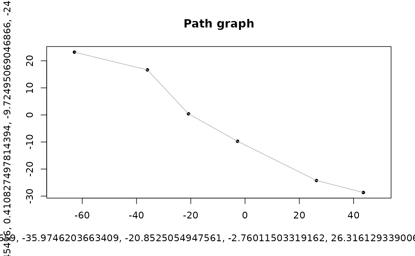
Quick plot for graph layouts — plot.layout • grip

For 2D layouts, draws vertices and edges using base graphics. For 3D layouts, the behaviour depends on the projection argument:

"rgl" (default): Opens an interactive rgl scene when that package is installed. Falls back to "ortho" with a warning if rgl is not available.
"ortho": Projects the 3D coordinates to 2D with project.3d and draws them with base graphics, giving a static figure suitable for vignettes and non-interactive reports.

Usage

# S3 method for class 'layout'
plot(x, ..., edges = NULL,
  projection = c("rgl", "ortho"), azimuth = 35, elevation = 22,
  vertex.col = "black", edge.col = "gray70")

Arguments

x: Numeric coordinate matrix with at least two columns.
...: For static plots, base graphics options override defaults, including asp, axis labels, limits, pch, cex, and vertex col/bg. In an orthographic plot, symbol, size, color, line width and type options are passed to points(); other options configure the plot region. Edges use edge.col. For interactive plots, options go to rgl::plot3d() and follow its conventions (for example size, not base-graphics cex).
edges: Optional two-column matrix of edges (1-based vertex ids).
projection: Character string controlling how 3D layouts are displayed: "rgl" (default) for an interactive rgl widget, or "ortho" for a static orthographic projection via base graphics. Ignored for 2D layouts.
azimuth: Rotation around the vertical axis in degrees. Only used when projection = "ortho". Default 35.
elevation: Rotation around the horizontal axis in degrees. Only used when projection = "ortho". Default 22.
vertex.col: Colour(s) for the vertices. Recycled to match the number of vertices. Default "black".
edge.col: Colour for the edges. Default "gray70".

Value

NULL (called for side effects).

Examples

edges <- cbind(1:5, 2:6)
coords <- grip(edges, n = 6, dim = 2,
                      placement = "barycenter",
                      rounds = 5, final_rounds = 5,
                      num_init = 3, num_nbrs = 4,
                      seed = 1)
plot.layout(coords, edges, main = "Path graph", pch = 16, cex = 0.8)