Finding your way around gflow

gflow studies scalar fields on graphs: where a field rises or falls, which vertices belong to a basin, and how changes in two fields align. Start with a task, then use the catalog to find its detailed help. The example graphs and fields introduce inspectable inputs. The canonical workflow covers construction and refinement in more detail; the noisy-circle workflow adds noisy observations, graph selection, and local association.

Two peaks on a seven-vertex path. The height-3 plateau joins the higher peak at field height 1; the tree records that relationship. Reproduce the analysis below.

Choose a starting point

Your task	Entry point	Worked route
Construct and compare basins	`create.basin.complex()`	First analysis and construction workflow.
Inspect hierarchy and support	`get.basin.merge.tree()`, `get.basin.table()`, `get.basin.membership()`	Path and grid examples; distinguish raw, retained and assigned supports.
Follow trajectories	`get.basin.trajectory.forest()`, `construct.madag()`	Canonical trajectory workflow.
Compare fields	`lcor()`, `lslope()`, `gfcor()`	Noisy-circle example and flow association.

For saved historical results, the secondary route is as.basin.complex(): reconstruction requires the original graph and an available construction field. The full catalog below retains the archive and advanced interfaces.

The method-parameter reference is also installed: help("basin-parameters", package = "gflow"). Its tables are generated from the constructor’s resolved defaults. In particular, CLOSEST requires exact connected plateaus, density modulation requires a supplied density, and disabled nondefault refinement settings can still be inapplicable.

Across interfaces, edge.length.list and the inherited weight.list both supply graph edge lengths, not vertex mass or affinity. lcor() defaults to ordinary differences for both fields; lslope() defaults to log-ratios for the response field. Set z.diff.type = "difference" explicitly for an ordinary response slope. The local statistic is an edge-difference cosine; interpreting it as a Euclidean gradient cosine requires isotropic local directions, as explained in help("lcor", package = "gflow").

A complete first analysis

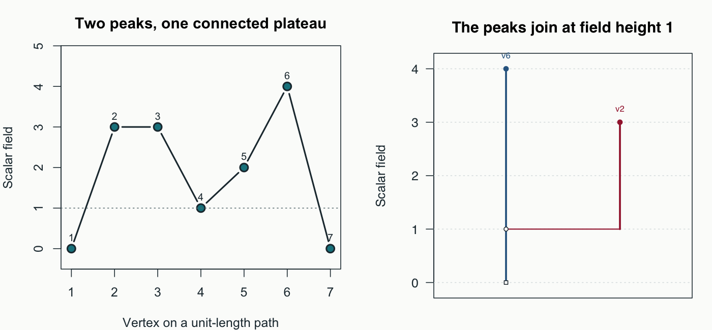
This seven-vertex path has a plateau at vertices 2–3 and a higher peak at vertex 6. No graph-construction package call or hidden workspace object is needed. Edge lengths are one distance unit; field values have arbitrary field units. Unit vertex masses express equal support, independently of field height.

library(gflow)
adjacency <- list(2L, c(1L, 3L), c(2L, 4L), c(3L, 5L),
                  c(4L, 6L), c(5L, 7L), 6L)
edge_lengths <- lapply(adjacency, function(v) rep(1, length(v)))
field <- c(0, 3, 3, 1, 2, 4, 0)
bc <- create.basin.complex(
  adj.list = adjacency, edge.length.list = edge_lengths, field = field,
  method = "superlevel_merge_tree", direction = "max",
  vertex.mass = rep(1, length(field))
)
stopifnot(identical(bc$status, "ok"))
tab <- get.basin.table(bc)
knitr::kable(tab[, c("extremum.vertex", "birth.level", "death.level",
                     "persistence", "raw.support.size")],
             caption = "Peak births and lifetimes on the seven-vertex path.")

Peak births and lifetimes on the seven-vertex path.
extremum.vertex	birth.level	death.level	persistence	raw.support.size
6	4	0	4	7
2	3	1	2	2

get.basin.membership(bc)
#>   vertex direction            basin.id membership.weight membership.status
#> 1      1       max basin_max_v00000006               1.0               raw
#> 2      2       max basin_max_v00000006               0.5               raw
#> 3      2       max basin_max_v00000002               0.5               raw
#> 4      3       max basin_max_v00000006               0.5               raw
#> 5      3       max basin_max_v00000002               0.5               raw
#> 6      4       max basin_max_v00000006               1.0               raw
#> 7      5       max basin_max_v00000006               1.0               raw
#> 8      6       max basin_max_v00000006               1.0               raw
#> 9      7       max basin_max_v00000006               1.0               raw
#>   source.stage is.primary vertex.id
#> 1 construction       TRUE         1
#> 2 construction      FALSE         2
#> 3 construction       TRUE         2
#> 4 construction      FALSE         3
#> 5 construction       TRUE         3
#> 6 construction       TRUE         4
#> 7 construction       TRUE         5
#> 8 construction       TRUE         6
#> 9 construction       TRUE         7
get.basin.assignment(bc)
#>   vertex direction            basin.id assignment.weight assignment.status
#> 1      1       max basin_max_v00000006                 1          assigned
#> 2      2       max basin_max_v00000002                 1          assigned
#> 3      3       max basin_max_v00000002                 1          assigned
#> 4      4       max basin_max_v00000006                 1          assigned
#> 5      5       max basin_max_v00000006                 1          assigned
#> 6      6       max basin_max_v00000006                 1          assigned
#> 7      7       max basin_max_v00000006                 1          assigned
#>   assignment.policy root.vertex next.vertex vertex.id root.vertex.id
#> 1    elder_at_merge           6          NA         1              6
#> 2    elder_at_merge           2          NA         2              2
#> 3    elder_at_merge           2          NA         3              2
#> 4    elder_at_merge           6          NA         4              6
#> 5    elder_at_merge           6          NA         5              6
#> 6    elder_at_merge           6          NA         6              6
#> 7    elder_at_merge           6          NA         7              6
#>   next.vertex.id
#> 1           <NA>
#> 2           <NA>
#> 3           <NA>
#> 4           <NA>
#> 5           <NA>
#> 6           <NA>
#> 7           <NA>
tree <- get.basin.merge.tree(bc, required = TRUE)
cut(tree, height = 2)$components
#>         component.id graph.component            basin.id            extremum.id
#> 1 component_max_0001               1 basin_max_v00000002 extremum_max_v00000002
#> 2 component_max_0002               1 basin_max_v00000006 extremum_max_v00000006
#>   extremum.vertex extremum.value support.size support.mass vertices vertex.ids
#> 1               2              3            2    0.2857143     2, 3       2, 3
#> 2               6              4            2    0.2857143     5, 6       5, 6

plot(tree, direction = "max", type = "tree", label = "extremum.vertex",
     show.mass = FALSE, show.support = FALSE)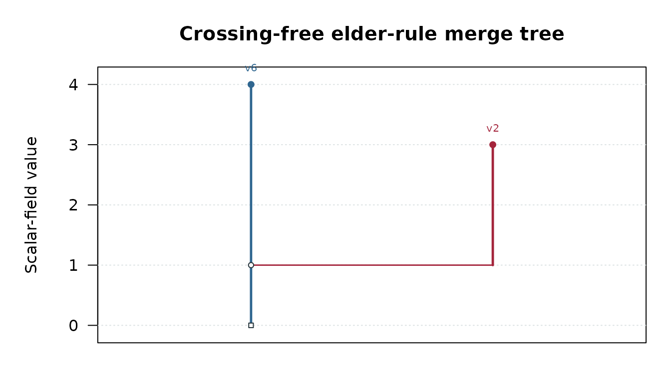

Ascending merge tree labeled by peak vertex. The plateau peak is born at 3 and joins the older peak at level 1; the component root spans levels 4 to 0.

The constructor accepts exactly the five full method strings in the next table. "merge_tree" is not an alias. Use edge.length.list and field; weight.list and f are not constructor aliases. Other functions, including lcor(), do use weight.list, so check the selected function’s help.

Inputs, directions, and method choices

For n vertices, adj.list[[i]][j] is the 1-based index of a neighbor of vertex i; edge.length.list[[i]][j] is the length of that same edge. Both lists have length n. Neighbors must be unique, in range, and different from the source vertex. Every edge needs a reverse edge of equal length (within graph.params$edge.length.symmetry.tolerance, an absolute tolerance). Lengths must be finite and nonnegative. Prefer positive lengths for derivative or inverse-length calculations. Use integer(0) and numeric(0) for an isolated vertex, rather than NULL.

The canonical validator accepts disconnected graphs and records components. Exact merge trees work component by component, including isolates. This does not guarantee that every backend and refinement can cover every component; inspect status, diagnostics, and uncovered membership for the chosen method. Never add artificial edges solely to hide disconnectedness.

Coordinates describe observation locations or a drawing. They are not an argument to the canonical constructor: adjacency and lengths define its geometry. field supplies one finite numeric value per vertex in graph order. It may be observed, known, or estimated elsewhere. vertex.id optionally preserves unique external IDs; indexing remains internal and 1-based, with external-ID companion columns in the returned tables.

vertex.mass is nonnegative empirical or quadrature support with positive total. The constructor normalizes it to sum to one for mass summaries and mass-threshold refinement; it does not infer uniform mass when omitted. Unavailable mass summaries are NA. Full support mass counts each containing basin, whereas raw.allocated.mass apportions mass using raw membership weights. Overlapping full support masses need not sum to one. vertex.density is a separate nonnegative field that changes trajectory edge scores only in density-modulated flow. Neither input estimates the other, and mass does not redefine the exact graph level-set hierarchy.

direction = "max" follows increasing field values and "min" decreasing values; "both" computes both orientations. Older help sometimes calls the support reached downward from a maximum a descending basin. Here direction always names the extremum toward which the analysis is oriented.

`method`	Basin definition and controls	Distinct output
`"trajectory_flow"`	`modulation = "CLOSEST"` contracts connected exact plateaus, then chooses an improving boundary edge by length, target vertex, and source vertex. Other modes are `"NONE"`, `"EDGELEN"`, `"DENSITY"`, `"DENSITY_EDGELEN"`; these do not use the exact-plateau contraction.	Trajectory forest, terminal supports, optional primary labels.
`"superlevel_merge_tree"`	Connected sets with `field >= height` for maxima, or `field <= height` for minima. Only `plateau.tolerance = 0` is supported. Equal births use the smaller representative vertex as elder.	Hierarchical supports, births, merge events, component roots, persistence.
`"geodesic_reachability"`	Monotone geodesic reachability from extrema, with `edge.length.quantile.thld` limiting edges. Its strict-extremum/plateau behavior differs from the exact level-set method.	Possibly overlapping and incomplete supports; optional stored trajectories in the backend record.
`"rtcb"`	Relaxed trajectory-constrained basins. Controls include candidate-region size `n.min`, cumulative monotonicity control `m.min`, tolerance controls `tau0`, `kappa`, and path limits `k.max`, `h.max`, `d.path.max`. Use the method’s own parameter definitions.	Constrained-path supports and recorded backend parameters; no canonical trajectory forest or backend primary assignment.
`"overlap_cell_complex"`	Requires `direction = "both"`. Merges basin overlaps using `basin.merge.overlap.thld`; three `min.*.cell.size.thld` controls filter ascending/descending and same-direction cells.	Cell summary, intersections, cluster mappings, complex graph, and simplified field.

RTCB means relaxed trajectory-constrained basins in the implemented backend. It searches a distance-limited candidate region and allows bounded cumulative movement against the desired direction. n.min limits the initial number of settled candidate vertices, not the retained basin size. m.min determines the loss-to-gain allowance; optional q.min takes precedence. run.max limits consecutive adverse steps; tau0 and kappa define a local tolerance schedule; k.max caps retained search labels per vertex, h.max caps path hops, and d.path.max caps path length. This is not a resampling or trajectory-voting procedure, despite the older guide’s “robust trajectory-consensus” wording.

For trajectory flow, edge.length.quantile.thld = 1 keeps the full edge-length range. Lower values interact with long.edge.fallback ("allow_and_flag", "allow", or "forbid"). store.trajectories and max.trajectory.length control recording. CLOSEST uses plateau.policy = "connected_exact"; other modulations require "none". A terminal plateau has no strictly improving neighbor, and its representative is its smallest vertex. Optional field perturbation uses tie.breaking = TRUE and an explicit tie.seed; it changes the construction field while preserving the caller’s random state. Record that choice when comparing exact ties.

The shared schema is a navigation and provenance contract, not a claim that these methods produce identical basins. Do not transfer parameters or infer statistical robustness from a method’s name. The overlap-cell backend also requires compatible dgraphs graph operations; a recoverable backend error returns status = "failed" with diagnostic text, rather than usable cells.

Read results through accessors

Check construction status before interpreting empty tables. Invalid inputs raise errors; a recoverable backend failure can instead return a failed object.

Accessor	Public schema and interpretation
`get.basin.table(bc)`	One row per basin: identity, `type`, `method`, `retained`, extremum vertex/value, `birth.level`, `death.level`, `persistence`, `parent.basin.id`; raw, retained, and primary support vertex lists, sizes, and masses; `raw.allocated.mass`, assignment and retention status. Non-applicable measures are `NA`.
`get.basin.membership(bc)`	Raw many-to-many rows: `vertex`, `direction`, `basin.id`, `membership.weight`, `membership.status`, `source.stage`, `is.primary`, and `vertex.id`. This is construction membership, not the refined support table.
`get.basin.assignment(bc)`	One row per vertex and requested direction when available: `basin.id`, weight, status, policy, `root.vertex`, `next.vertex`, and external-ID companions. `NA` labels with `not_applicable` mean no policy/result, not necessarily uncovered vertices.
`get.basin.merge.tree(bc)`	`basin.merge.tree` for the exact level-set method, otherwise `NULL`. Its documented `merge.table` records losing/surviving basins, merge plateau/vertices, level, persistence, and event status.
`get.basin.trajectory.forest(bc)`	For trajectory flow: named `next.vertex` and `root.vertex` vectors by direction, trajectories, recording status, modulation, plateau and tie controls. Reachability/RTCB recording does not create this canonical forest.
`get.basin.cells(bc)`	For overlap-cell construction: `cell.summary` (`family`, `cell.id`, `n.vertices`, `vertices`), `cells`, `basin.intersections`, `complex.graph`, `cluster.assignments`, `cluster.mappings`, `simplified.field`. Other methods return `NULL`.

Use required = TRUE on the three structure accessors to reject absent structures. Use summary(bc) for direction-specific ranking and availability information; the printed summary includes a bounded ranking and separate raw, retained, and assigned vertex coverage. as.data.frame(bc) gives the basin table. plot(bc) shows the input field against vertex index. Select view = "merge_tree" for the exact hierarchy, or supply an n by 2 coordinates matrix to view = "assignment" or view = "overlap". Choose direction explicitly if both were constructed. Failed construction is labeled in the input-field view and rejected by analytical views; partial results warn. These plots do not modify the analysis. basin() and basins() also dispatch on canonical objects, but the non-colliding get.basin.*() accessors make the intended schema explicit.

A vertex can be in multiple supports. Equal-share membership weights encode overlap; they are not posterior probabilities. To find raw uncovered vertices in a direction, subtract its membership vertices from seq_along(field). For refined coverage use the union of the table’s retained support vertex lists. Do not infer coverage from assignment alone. The "largest_membership_then_extremum" assignment policy resolves eligible membership using the implementation’s size/extremum ordering. It is available for trajectory and reachability methods. Reachability defaults to "none"; RTCB currently records "none" even if "backend_primary" was requested. Overlap cells have no primary assignment. Exact trees use "elder_at_merge".

For an ascending merge tree, a branch is born at a maximum and dies when its component joins an older branch as the height decreases. Persistence is birth.level - death.level. For descending trees the height increases from minima and persistence is death.level - birth.level. Both are nonnegative and in field units. Each disconnected component has a surviving root whose death is its opposite field extreme; a constant component has zero lifetime. This finite root convention is not an observed merger into another component. Hierarchical support can include child support, whereas primary assignment keeps branch labels. Neither is the same as an exact level-set cut: cut(tree, height, direction) returns active components and their membership. Persistence measures lifetime across field thresholds, not a p-value or an automatic significance test. as.dendrogram(tree, direction, component) and plot(tree, ...) are views of this hierarchy.

Refine or convert a basin analysis

Use simplify.params in the constructor. The fixed order is relative-value filtering, maxima/minima clustering, geometric filtering, support filtering, then expansion. Filtering changes retained flags/support and clears affected assignments; clustering unions retained supports and remaps assignments; expansion adds vertices to retained supports. Raw membership rows, weights, and their mass allocation survive refinement; is.primary is refreshed where a current assignment matches a raw row. It cannot describe vertices added to retained support. Inspect current primary labels with the assignment accessor.

Relative-value, clustering, and geometric stages apply to trajectory flow, reachability, and RTCB. Support filtering also applies to exact trees. Expansion applies only to reachability and RTCB; overlap cells have their own construction controls and reject canonical refinement stages. Positive min.basin.mass requires supplied mass. Resolved controls are in parameters; provenance$refinement.stages records stages, before/after counts, and snapshots. The example vignette shows why retained and raw supports must be read separately.

as.basin.complex() leaves a canonical input canonical. For archived gfc.flow, basins_of_attraction, or basin_cx, it reconstructs a canonical analysis from the supplied original adjacency/length lists and an available field. It does not simply relabel an old object or promise identical results. gfc.flow uses its stored y; basin_cx uses original_y; basins_of_attraction uses stored y or requires explicit field and permits method = "geodesic_reachability" or "rtcb". Review method/refinement controls instead of assuming all archived settings are inferred. Conversion provenance records reconstruction and preserves the archived object.

Extrema, trajectories, and harmonic coordinates

detect.adaptive.extrema() expands graph neighborhoods subject to max.radius and min.neighborhood.size and returns gflow_local_extrema. Equal field values stop the adaptive detector’s strict comparison, and its neighborhood count excludes the center. It can accept a smaller neighborhood before a more extreme vertex farther away. It differs from the fixed-radius dgraphs::detect.local.extrema() and that function’s local_extrema class: that detector uses the full radius, permits equal values, and includes the center in its neighborhood count. vertices(result) uses the shared dgraphs::vertices() generic and dispatches on the object’s class; for gflow adaptive extrema, include.center = TRUE includes the center exactly once. Neither detector should be substituted for exact plateau merge-tree births.

For individual directed paths, construct.madag() builds a monotonic ascent directed acyclic graph (MADAG): vertices and edges reachable by strictly increasing paths from a source. A directed acyclic graph has no directed cycles. madag.bottlenecks() reports vertices shared by enough paths to a chosen sink. Limit path enumeration for large graphs. A basin-intersection graph from construct.gflow.graph() instead has a vertex for each archived basin and edges for shared support; it is not the original directed flow graph.

compute.harmonic.extension() fixes arc-length positions on a supplied path and solves for neighboring coordinates that average their neighbors. Its tube radius counts hops or shortest-path distance, according to tube.type. With use.edge.weights = TRUE, inverse edge lengths supply the averaging weights. Inspect n.iterations and final.max.change; this operation extends a path coordinate, not a statistical response model. apply.harmonic.extension() and comparison helpers operate on their own local-subgraph records. Plotting and file-saving defaults differ: disable visualization/saving when only numerical results are needed.

Local association and inference

lcor() compares the vectors of field differences from each vertex to its neighbors using a normalized inner product. It is symmetric when fields and their transformation controls are exchanged. type = "derivative" weights by inverse squared edge length; "unit" uses equal weights; "sign" retains direction agreement. hop.radius > 1 uses vertices reachable within that many hops and, for derivative weighting, shortest lengths within the hop limit. This is local alignment of graph differences, not an ordinary Pearson correlation of observations in a neighborhood.

Inputs (rows are vertices)	`lcor()` result, without instrumentation	`lslope()` result
Vector and vector	Length-`n` coefficients	Length-`n` coefficients
Vector and matrix, or matrix and vector	`n` by number-of-columns matrix	Vector directing field plus response matrix is supported; matrix directing field plus vector is rejected.
Two different matrices	`n` by `ncol(y)` by `ncol(z)` array	All directed pairs in the same array shape
Identical matrices	`n` by number-of-unordered-pairs matrix, excluding diagonal	All directed pairs; no symmetric shortcut

Numeric data frames are converted to matrices. instrumented = TRUE exposes diagnostics where supported; use the documented result fields rather than assuming that a plain matrix is a list. Keep mc.cores = 1L for portable matrix-pair computations.

lslope() chooses an improving edge by the largest field difference in the requested direction, then measures change in z relative to change in y. This current edge selection is based on field differences, not their ratio to edge length. At extrema without an improving edge the reported coefficient is zero. type = "slope" has response-units per directing-field-unit; "normalized" compresses the ratio, and "sign" keeps its sign information. For ordinary signed continuous fields explicitly set both difference types to "difference": lslope() defaults to "logratio". Log ratios require values compatible with the positive pseudocount transformation. lslope.neighborhood() accepts two vectors and uses all incident differences in a weighted regression through the origin, returning coefficients, local scales, and local correlation. None of these functions requires a fitted model.

response <- 2 * field + 1
data.frame(
  vertex = seq_along(field),
  alignment = as.numeric(lcor(adjacency, edge_lengths, field, response)),
  directed.slope = as.numeric(lslope(
    adjacency, edge_lengths, field, response,
    y.diff.type = "difference", z.diff.type = "difference"))
)
#>   vertex alignment directed.slope
#> 1      1         1              2
#> 2      2         1              0
#> 3      3         1              0
#> 4      4         1              2
#> 5      5         1              2
#> 6      6         1              0
#> 7      7         1              2

An association estimate, a permutation test, and a posterior summary answer different questions:

permutation.test.lcor() holds adjacency and edge lengths fixed and recomputes local correlations and a feature summary on every permutation. permute = "z" applies one common row permutation to all feature columns, preserving their within-row relationships; "y" permutes the response. It does not reconstruct graphs, refit fields, or reselect neighborhoods. Only its exposed difference/weighting controls are forwarded; there is no hop.radius argument in this test. Its statistics are "mean.abs", "max.abs", and the upper-tail signed "mean". The Monte Carlo p-value is (1 + number at least as large as observed) / (n.perm + 1).
That test requires exchangeability of the permuted vertex rows under the null, conditional on the held-fixed inputs. Spatial dependence, repeated subjects, or a graph selected using the tested fields can invalidate unrestricted permutation. No block/stratum permutation control is exposed. q.value is the Benjamini–Hochberg adjustment across feature tests, not vertex-wise testing. False discovery rate control requires valid p-values and the procedure’s independence or suitable positive-dependence conditions. Increasing permutation count improves resolution, not exchangeability.
lcor.with.posterior() takes a fixed y.hat and supplied n by B field draws, or a list of such matrices for multiple features. All fields must be finite numeric values and all features must have the same positive draw count; inconsistent counts are rejected before computation. Supplied feature names are preserved, and supplied vertex names must agree in order (see help("lcor.with.posterior", package = "gflow")). It computes local correlation for each draw and returns feature-by-vertex means, standard deviations, and equal-tail quantile intervals. The graph and response remain fixed. It fits no posterior model and does not propagate uncertainty absent from those inputs. Intervals are pointwise, not simultaneous; their posterior interpretation depends on how the draws were obtained.

Flow-aware association: current input boundary

gfcor() now accepts two successful canonical trajectory_flow complexes, each built with direction = "both". Choose support.stage = "raw" or "retained" explicitly. Retained association supports only support filtering; other refinement choices and other method families are rejected. The graph, lengths, external vertex IDs and order must match, and the supplied fields must be the construction values. Canonical masses are normalized to sum one, with uniform mass by default. Archived basins_of_attraction inputs remain supported with their original behavior; the retired constructor remains retired.

adj.assoc <- list(2L, c(1L, 3L), c(2L, 4L), c(3L, 5L), 4L)
lengths.assoc <- lapply(adj.assoc, function(v) rep(1, length(v)))
y.assoc <- c(0, 3, 1, 2, 0)
by <- gflow::create.basin.complex(adj.assoc, lengths.assoc, y.assoc,
    method = "trajectory_flow", direction = "both")
bz <- gflow::create.basin.complex(adj.assoc, lengths.assoc, -y.assoc,
    method = "trajectory_flow", direction = "both")
gflow::gfcor(y.assoc, -y.assoc, by, bz, support.stage = "raw")
#> Gradient Flow Correlation Analysis
#> ===================================
#> 
#> Canonical trajectory supports: raw
#> Global summaries use 5/5 valid vertices (normalized mass 1.0000).
#> 
#> Global Association Measures:
#>   Polarity concordance (A_pol):  -1.0000
#>   Sign concordance (kappa_pol):  -1.0000
#> 
#> Vertex Counts:
#>   Positive association: 0
#>   Negative association: 5
#>   Zero association:     0
#>   Invalid (flat or uncovered): 0
#> 
#> Basin Structure:
#>   Y maxima: 2, Y minima: 3
#>   Z maxima: 3, Z minima: 2
#> 
#> Settings: polarity.scale = 'value', epsilon = 1.00e-10

Reversing the field produces negative polarity concordance. Self-association averages squared polarity and need not equal one. Check validity flags and coverage: invalid vertices are omitted from global averages, while numeric zeros remain as placeholders. The canonical metadata maps zero-based kernel basin positions to stable basin IDs.

gfassoc.membership() divides a vertex’s membership equally among its containing basins and forms maximum/minimum cell memberships. Its basin/cell index arrays are 0-based positions, unlike its 1-based extremum vertices. gfassoc.polarity() combines these memberships with one field to locate each vertex between accessible minima and maxima. "value" uses normalized height; "rank" uses within-cell ranks. Invalid or flat ranges are marked, and should not be read as zero association.

gfcor() aggregates products of the two polarity coordinates at vertex, basin, and global levels. A_pol is mean polarity concordance and kappa_pol summarizes sign concordance. Its confidence field is absolute association magnitude, not a calibrated confidence probability. Unlike the canonical constructor, gfcor() defaults to uniform aggregation weights if mass is absent. gfassoc.overlap() sums products of soft memberships with optional vertex mass. gfassoc.deviation() compares an overlap matrix with its row/column marginal-product expectation and returns residuals; it does not perform a permutation or chi-squared test. These summaries describe supplied structures; association does not establish causation.

Function catalog

The catalog covers 112 explicit exports: 111 locally defined functions and one dependency re-export. There are also 99 S3 registrations, including three names that are explicitly exported as well. Each explicit export appears exactly once below. Start means a recommended entry point; Advanced means a working specialized interface with its own input schema, not a claim of validation for every dataset; Archive means an interface to older objects or their component records; Retired means an exported function that raises a migration error. These labels distinguish availability from recommendation. Open exact arguments with help("function.name", package = "gflow").

Basin construction and conversion

Function	Purpose	Status
`create.basin.complex()`	Construct a canonical basin analysis with a chosen method.	Start
`as.basin.complex()`	Validate a canonical object or reconstruct from a supported archive.	Start
`compute.basins.of.attraction()`	Retired reachability constructor; use canonical `geodesic_reachability`.	Retired
`compute.gfc()`	Retired composite refinement workflow; translate controls into canonical construction/refinement.	Retired
`compute.gfc.trajectory()`	Retired trajectory constructor; use canonical `trajectory_flow`.	Retired
`compute.gfc.flow()`	Retired trajectory alias; it also raises a migration error.	Retired
`create.basin.cx()`	Retired overlap constructor; use canonical `overlap_cell_complex`.	Retired
`compute.gfc.basins()`	Compute a specialized modulated-flow basin record (`gfc_basins`).	Advanced
`find.gflow.basins()`	Find path-based graph basins with size and edge controls.	Advanced
`create.gflow.cx()`	Construct an extrema-oriented complex with iterative harmonic modification.	Advanced
`create.morse.smale.complex()`	Construct a separate two-dimensional grid complex from `f.grid`.	Advanced

Stable accessors and summaries

Function	Purpose	Status
`get.basin.table()`	Read raw, retained, and primary basin summaries.	Start
`get.basin.membership()`	Read raw construction membership, including overlaps.	Start
`get.basin.assignment()`	Read current optional single-basin labels and their status.	Start
`get.basin.merge.tree()`	Extract the exact level-set hierarchy.	Start
`get.basin.trajectory.forest()`	Extract canonical trajectory-flow paths and successor/root records.	Start
`get.basin.cells()`	Extract overlap-cell structures and summary.	Start
`basin()`	Generic for one basin; canonical and historical classes dispatch differently.	Advanced
`basins()`	Generic for basin collections; consult the object’s method.	Advanced
`get.basin()`	Find a labeled basin in an archived `gfc.flow`.	Archive
`get.gflow.build.identity()`	Report the loaded package build and manifest identity.	Advanced

Extrema and merge trees

Function	Purpose	Status
`detect.adaptive.extrema()`	Detect extrema with adaptive graph neighborhoods.	Start
`find.critical.points()`	Identify critical points on a two-dimensional field grid.	Advanced
`find.local.extrema()`	Find labeled extrema with graph-basin size controls.	Advanced
`compute.extrema.hop.nbhds()`	Compute extrema-centered hop neighborhoods.	Advanced
`get.nbrs()`	Extract an extrema-neighborhood component by label.	Advanced
`relabel.extrema()`	Reorder and label an extrema data frame.	Advanced
`compute.persistence()`	Run the older persistence/basin calculation with `n.top.basins` and `alpha`; not a canonical tree accessor.	Advanced
`plot.basin.merge.tree()`	Tree/barcode view; normally call `plot(tree)`.	Start
`cut.basin.merge.tree()`	Exact field-height query; normally call `cut(tree, height)`.	Start
`as.dendrogram.basin.merge.tree()`	Coerce one direction/component; normally call `as.dendrogram(tree)`.	Advanced
`get.basin.merge.tree.layout()`	Obtain validated tree drawing coordinates.	Advanced
`extremality.summary()`	Summarize extremality scores in a domain-complex record.	Advanced
`compute.pextrema.nbhds()`	Extract neighborhoods from extremality and degree criteria.	Advanced
`maxp()`	Evaluate a neighborhood-weighted maximum score from `y` and `rho`.	Advanced
`minp()`	Evaluate a neighborhood-weighted minimum score from `y` and `rho`.	Advanced
`analyze.extrema.distribution()`	Inspect extrema distributions and candidate filtering thresholds.	Advanced
`classify.spurious.extrema()`	Classify extrema by supplied heuristic criteria.	Advanced
`compare.retained.extrema()`	Compare extrema retained by selected thresholds.	Advanced
`create.hop.nbhd.extrema.df2()`	Tabulate hop-neighborhood extrema and heuristic classifications.	Advanced
`suggest.threshold()`	Suggest extrema thresholds from expected count/range controls.	Advanced

“Spurious,” “probability,” and “persistence” in older function names do not by themselves imply a calibrated statistical test. Prefer the exact canonical tree for graph level-set births and mergers.

Function	Purpose	Status
`cluster.local.extrema()`	Cluster overlaps in an archived basin object.	Archive
`filter.basins()`	Retain selected extrema in an archived basin object.	Archive
`filter.basins.by.relvalue()`	Filter an archived basin object by relative field value.	Archive
`expand.basins.to.cover()`	Expand supplied basin vertex lists along the graph.	Advanced
`generate.refinement.report()`	Format a report from an older composite-refinement record.	Archive
`replace.basin.label()`	Replace a label in a graph-gradient-flow record.	Archive
`uncovered.vertices.gfc.flow()`	Locate uncovered vertices in an archived trajectory-flow result.	Archive
`count.feature.carriers()`	Count features present in a selected matrix row subset.	Advanced
`set.boundary()`	Find boundary vertices of a supplied subset using adjacency.	Advanced

Trajectories, cells, and flow graphs

Function	Purpose	Status
`construct.madag()`	Build monotonic ascent paths from a source, with enumeration limits.	Advanced
`madag.bottlenecks()`	Find vertices shared by a chosen fraction of paths to a sink.	Advanced
`construct.gflow.graph()`	Build an intersection graph from archived merged basins.	Archive
`construct.graph.gradient.flow()`	Compute a scale-controlled graph-gradient-flow record.	Advanced
`compute.graph.gradient.flow()`	Compute flow information with supplied extrema lists.	Advanced
`compute.gfc.modulation()`	Compute graph edge modulation weights from density/length controls.	Advanced
`build.se.tree()`	Build a spurious-extrema tree from a source and classified extrema/basins.	Advanced
`extract.gradient.trajectory()`	Extract a path from an archived basin trajectory record.	Archive
`extract.cell.trajectory()`	Join minimum/maximum paths through an archived cell vertex.	Archive
`vertex.cell.trajectory.gfc.flow()`	Extract a vertex’s trajectory inside an archived flow cell.	Archive
`filter.cells.by.criteria()`	Filter a gradient-flow-cell record by counts or percentiles.	Archive
`filter.cells.by.vertex.count()`	Filter a gradient-flow-cell record by support size.	Archive
`cell.y.values()`	Extract response values for a supplied partition’s super-cells.	Advanced
`compute.tube.lens.corridor()`	Find graph corridors constrained by path length/excess.	Advanced
`construct.path.through.waypoints()`	Join waypoint vertices using a supplied igraph graph.	Advanced
`trajectory.distances.to.vertex()`	Measure path distances to a target vertex.	Advanced
`vertex.distances.to.trajectory()`	Measure distances from vertices to a path.	Advanced
`fit.trajectory.smooth.splines()`	Smooth mean/median trajectory coordinates in a 3D embedding.	Advanced
`graph.constrained.gradient.flow.trajectories()`	Follow a field using supplied graph/core-graph structures.	Advanced
`compute.gradient.trajectory()`	Follow a trajectory on a two-dimensional field grid.	Advanced
`compute.morse.smale.cells()`	Compute the cells of a two-dimensional field grid.	Advanced

Harmonic extension

Function	Purpose	Status
`compute.harmonic.extension()`	Extend arc-length coordinates from a path into its graph tube.	Start
`select.max.density.trajectory()`	Select the supplied path with greatest mean density.	Advanced
`apply.harmonic.extension()`	Apply a selected harmonic scheme to a local-subgraph record.	Advanced
`analyze.harmonic.extensions()`	Analyze extensions around supplied extrema and predictions.	Advanced
`compare.harmonic.methods()`	Compare numerical extensions on one local-subgraph record.	Advanced
`visualize.smoothing.steps()`	Visualize recorded complex-smoothing iterations.	Advanced

Local association

Function	Purpose	Status
`lcor()`	Estimate symmetric local alignment of field differences.	Start
`lslope()`	Estimate directed response on a chosen improving edge.	Start
`lslope.neighborhood()`	Regress incident response differences on directing-field differences.	Start
`permutation.test.lcor()`	Test feature-level local-correlation summaries by unrestricted row permutation.	Advanced
`lcor.with.posterior()`	Summarize local correlation over supplied field draws against a fixed response.	Advanced

Flow-aware association

Function	Purpose	Status
`gfcor()`	Summarize polarity concordance for canonical trajectory or archived basin objects.	Advanced
`gfassoc.membership()`	Normalize canonical trajectory or archived basin memberships.	Advanced
`gfassoc.polarity()`	Compute value/rank polarity from a field and compatible membership record.	Advanced
`gfassoc.overlap()`	Compute mass-weighted overlap between compatible membership records.	Advanced
`gfassoc.deviation()`	Describe residuals from marginal-product expected overlap.	Advanced

Domain-specific visualization and supporting grid tools

The three extrema-labeling functions add labels/segments to an existing native rgl scene and return invisibly; they do not return ivue widgets. Optional ivue scene layers are a separate rendering workflow and are not needed for these static examples. draw.basin() also adds to a native scene; its current implementation looks up a free graph.3d object rather than accepting coordinates explicitly, so it is not a self-contained new-analysis entry point. Grid utilities here support the separate two-dimensional Morse–Smale workflow; they are not a general synthetic-data API.

Function	Purpose	Status
`label.extrema.3d()`	Add extrema labels to a native 3D scene using supplied coordinates.	Advanced
`label.extrema.leaders.3d()`	Add extrema labels and leader segments to a native 3D scene.	Advanced
`label.extremality.3d()`	Add extremality-based labels to a native 3D scene.	Advanced
`draw.basin()`	Add archived basin vertices to a native 3D scene.	Archive
`critical.points.plot()`	Draw critical points in two dimensions.	Advanced
`grid.critical.points.plot()`	Draw grid extrema with coordinate axes.	Advanced
`function.contours.plot()`	Draw contours of a grid field.	Advanced
`gradient.trajectory.plot()`	Draw one ascending/descending grid trajectory.	Advanced
`gradient.trajectories.plot()`	Draw a collection of grid trajectories.	Advanced
`morse.analysis.plot()`	Combine contours, critical points, and a grid trajectory.	Advanced
`morse.smale.cells.plot()`	Draw two-dimensional grid cells.	Advanced
`morse.smale.complex.plot()`	Draw a grid complex from a supplied function.	Advanced
`morse.smale.complex.plot.from.critical()`	Draw a grid complex using supplied critical points.	Advanced
`separatrices.with.cells.plot()`	Draw cell-separating curves and regions in a specified 2D layout.	Advanced
`create.grid()`	Prepare a coordinate grid for the two-dimensional workflow.	Advanced
`evaluate.function.on.grid()`	Evaluate a supplied function into a grid matrix.	Advanced
`evaluate.function.on.grid.as.vector()`	Evaluate a supplied function in grid vertex order.	Advanced
`create.lmin.lmax.labels()`	Label domain-complex extrema using supplied state/taxonomy data.	Advanced
`create.lmin.lmax.label.indicators()`	Build label tables and indicators for domain-complex extrema.	Advanced
`create.lmin.lmax.contingency.table()`	Tabulate relationships between labeled extrema.	Advanced
`morse.smale.complex.lmin.lmax.summary()`	Summarize a supplied domain-complex and its feature annotations.	Advanced
`prof.fn()`	Profile a selected feature against supplied similarity/taxonomy records.	Advanced
`find.longest.true.stretch()`	Locate the longest consecutive TRUE run in a logical vector.	Advanced
`elapsed.time()`	Format elapsed computation time.	Advanced

Dependency re-export

Function	Purpose	Status
`vertices()`	Re-export of `dgraphs::vertices()`: shared generic dispatches to each package’s object methods.	Re-export

Generic methods and object workflows

R’s S3 dispatch selects a method from an object’s class when a generic is called. For canonical basins use print(), summary(), plot(), as.data.frame(), basin(), and basins(). For exact trees use plot(), cut(), and as.dendrogram(). Those last three method names are also explicit exports and occur once each in the catalog, not twice.

Use print()/summary() on local-association, harmonic, adaptive-extrema, and MADAG results as available. The remaining registrations below record historical or specialized schemas; their presence does not make them canonical entry points. In particular, names such as basin.trajectories are S3 registrations, not independent constructors. Some historical generics (list.cells, cell.trajectories, lmax, and others) are internal and should not be used as new public workflows. Class names are shown here only to make dispatch and coverage inspectable.

Generic	Registered classes
`as.basin.complex`	`basin_complex`, `basin_cx`, `basins_of_attraction`, `default`, `gfc.flow`
`as.data.frame`	`basin_complex`, `harmonic_extension`
`as.dendrogram`	`basin.merge.tree`
`basin`	`basin_complex`, `basins_of_attraction`, `cx.merge`, `feature.carriers`, `prev.eval`, `trajectories`, `trajectories.gfc.flow`, `vertices`
`basins`	`basin_complex`, `basins_of_attraction`, `merge`, `union`
`cell.trajectories`	`gfc.flow`, `max.edge.length`, `monotonicity`
`cut`	`basin.merge.tree`
`identify`	`gradient.flow.cells`
`list.basins`	`default`, `gfc.flow`
`list.cells`	`default`, `gfc.flow`
`lmax`	`basin_summary`, `basins`
`lmin`	`basin_summary`, `basins`
`merge`	`clustered.basins`, `gfc.basins`, `gfc.flow.basins`, `two.basins`, `two.extrema`
`plot`	`basin.merge.tree`, `basin_complex`, `basin_cx`, `feature.prevalence`, `gfc_modulation`, `gflow_graph`, `gflow_local_extrema`, `graphMScx`, `morse.smale.trajectories.from.point`
`print`	`basin_complex`, `basin_cx`, `basins_of_attraction`, `gfc.flow`, `gfc_basins`, `gfc_cell_trajectories`, `gfc_modulation`, `gfcor`, `gflow_cx`, `gflow_graph`, `gradient_flow_cells`, `harmonic_extension`, `lcor.posterior`, `lcor_permutation_test`, `lcor_matrix_matrix_result`, `lcor_vector_matrix_result`, `lslope_gradient_result`, `lslope_matrix_matrix_result`, `lslope_neighborhood_result`, `lslope_vector_matrix_result`, `madag`, `se_tree`, `summary.basin_complex`, `summary.basin_cx`, `summary.gfc_basin_trajectories`, `summary.gfc_cell_trajectories`, `summary.gfcor`, `summary.gflow_basins`, `summary.gflow_graph`, `summary.gflow_local_extrema`, `summary.ggflow`, `summary.lcor.posterior`
`show.basin`	`basin_cx`
`summary`	`basin_complex`, `basin_cx`, `basins_of_attraction`, `gfc.flow`, `gfc_basin_trajectories`, `gfc_cell_trajectories`, `gfcor`, `gflow_basins`, `gflow_graph`, `gflow_local_extrema`, `ggflow`, `gradient_flow_cells`, `lcor.posterior`, `lcor_matrix_matrix_result`, `lcor_vector_matrix_result`, `lslope_matrix_matrix_result`, `lslope_vector_matrix_result`, `madag`
`vertices`	`feature.carriers`, `gflow_local_extrema`

Migration and package boundaries

These instructions are available in installed help as help("gflow-migration", package = "gflow"), as well as here.

Earlier call or family	Current action
`detect.local.extrema()` in gflow	Use `gflow::detect.adaptive.extrema()` and recompute saved objects with the new class. The dgraphs detector has different semantics.
The five retired basin constructors	Use `create.basin.complex()` with the method and named parameter lists documented above; convert compatible archives with `as.basin.complex()`. No exact equivalence for every old argument combination is promised.
Generic graph construction, conversion, paths, and diagnostics	Use the documented public `dgraphs` API, with its current graph input/output schema. For example, `dgraphs::create.path.graph()` constructs a path; `dgraphs::detect.graph.endpoints()` handles endpoint diagnostics.
Generic graph layout	Use the appropriate layout package, for example optional `grip` for its documented layouts. A drawing is separate from the graph/field used for analysis.
Generic 3D rendering	Use `ivue::plot3D.plain()`, `ivue::plot3D.cont()`, `ivue::plot3D.groups()`, and scene layers such as `ivue::layer3D.path()` and `ivue::layer3D.edges()`.
Archived response smoothing / conditional-expectation estimators	`gflowx` is the archive for reproducing those analyses. Current `geosmooth` is a separate smoothing package, not an automatic drop-in replacement for every retired function.
Removed one-dimensional model-averaging functions (`magelo`, `mabilo`, `fit.pwlm*`, related families)	Extracted to `malo`; gflow no longer provides forwarders. Check that package’s public help for the specific estimator.
PHATE, diffusion/potential pseudotime, quadratic-form geodesics, random-walk smoothing experiments	Removed from the gflow API. No supported successor is claimed here.
Removed generic weighted-p-value helpers and `fassoc*` tests	No public core adapter. Choose an inferential procedure for the actual estimand; flow-aware descriptive summaries are not replacement tests.

Do not assume a renamed dependency function accepts the same object or arguments. These package boundaries do not require installing sibling packages to run the examples in this guide.

Find detailed help

help(package = "gflow")
help("gflow-package", package = "gflow")
help("create.basin.complex", package = "gflow")
help("gflow-migration", package = "gflow")
vignette("function-guide", package = "gflow")
vignette("example-graphs-and-fields", package = "gflow")

The task-first map and short purpose tables take inspiration from Hmisc’s documentation and its package overview and linked help. The categories and descriptions here follow gflow’s own objects and tasks.