Noisy Circle: End-to-End gflow Workflow
Source:vignettes/noisy_circle_core_workflow_vignette.Rmd
noisy_circle_core_workflow_vignette.RmdOverview
For a task map, see Finding your way around gflow. For tiny deterministic inputs, see Example graphs and fields.
This vignette follows one graph-centered analysis story. We start with noisy samples from a circle and a noisy response field over that circle. We then construct graph scales, visualize a selected graph, recover local extrema/basins from the response, and test local associations with permutation-based inference.
1) Simulate Geometry and Response
n <- 250L
radius <- 1

set.seed(11)
theta.obs <- runif(n, 0, 2 * pi)
X <- cbind(
  x = radius * cos(theta.obs) + rnorm(n, sd = 0.15),
  y = radius * sin(theta.obs) + rnorm(n, sd = 0.15)
)

# Response: a mixture of two circular Gaussian peaks (one larger, one smaller)
mu1 <- 0.80
mu2 <- 3.95
sd1 <- 0.30
sd2 <- 0.48
amp1 <- 1.40
amp2 <- 0.75

periodic.gaussian <- function(x, center, scale) {
  distance <- pmin(
    (x - center) %% (2 * pi),
    (center - x) %% (2 * pi)
  )
  exp(-(distance^2) / (2 * scale^2))
}
comp1 <- amp1 * periodic.gaussian(theta.obs, mu1, sd1)
comp2 <- amp2 * periodic.gaussian(theta.obs, mu2, sd2)
y.true <- comp1 + comp2
y <- y.true + rnorm(n, sd = 0.10)

theta.true <- seq(0, 2 * pi, length.out = 300)
circle.true <- cbind(
  x = radius * cos(theta.true),
  y = radius * sin(theta.true)
)
op <- par(mar = c(2.5, 2.5, 0.5, 0.5), mgp = c(2.5, 0.5, 0), tcl = -0.3)
plot(X, asp = 1, las = 1, xlab = "", ylab = "")
lines(circle.true, lwd = 2)
legend("topleft",
       legend = c("Observed samples", "True circle"),
       pch = c(1, NA),
       lty = c(NA, 1),
       col = c("black", "black"),
       bty = "n", cex = 0.9)
Observed samples around the known generating circle. Coordinate noise changes the graph geometry independently of response noise.
par(op)2) Build Graphs Across k
k.min <- 5L
k.max <- 12L

X.graphs <- dgraphs::create.iknn.graphs(
  X,
  kmin = k.min,
  kmax = k.max,
  max.path.edge.ratio.deviation.thld = 0.1,
  n.cores = 1L,
  verbose = TRUE
)
#>  Running single-threaded.
#> Processing k values from 5 to 12 for 250 vertices
#> Requested parallel.mode: auto
#> Parallel mode: serial
#> Starting graph processing
#> [compute_knn] running...[compute_knn] 0.001s
#> [graph_build/geometric_prune/isize_prune] running...[graph_build/geometric_prune/isize_prune] 0.131s
#> Graph processing completed (0.132)
#> [compute_knn] 0.001s
#> [graph_build] 0.006s
#> [geometric_prune] 0.125s
#> [isize_prune] skipped (with.isize.pruning=FALSE)
#> Creating return list objects ... DONE (0.000)
#> Total elapsed time (0.133)
summary(X.graphs)
#> Summary of iknn_graphs object
#> ----------------------------
#> Number of vertices: 250
#> k range: 5 to 12
#> Max path-edge ratio deviation threshold: 0.1
#> Path-edge ratio percentile: 0.5
#> Graph type: geometrically pruned
#>
#>  idx  k n_ccomp edges mean_degree min_degree max_degree sparsity
#>    1  5       1   852        6.82          2         15  0.97263
#>    2  6       1  1034        8.27          2         16  0.96678
#>    3  7       1  1189        9.51          2         20  0.96180
#>    4  8       1  1389       11.11          3         25  0.95537
#>    5  9       1  1546       12.37          3         28  0.95033
#>    6 10       1  1691       13.53          4         31  0.94567
#>    7 11       1  1831       14.65          4         32  0.94117
#>    8 12       1  2000       16.00          4         34  0.93574
3) Select Graph Scale
X.graphs2 <- dgraphs::build.iknn.graphs.and.selectk(
  X,
  kmin = k.min,
  kmax = k.max,
  method = "edit",
  n.cores = 1L,
  verbose = TRUE
)
#>  Running single-threaded.
#> Processing k values from 5 to 12 for 250 vertices
#> Requested parallel.mode: auto
#> Parallel mode: serial
#> Starting graph processing
#> [compute_knn] running...[compute_knn] 0.001s
#> [graph_build/geometric_prune/isize_prune] running...[graph_build/geometric_prune/isize_prune] 0.132s
#> Graph processing completed (0.132)
#> [compute_knn] 0.001s
#> [graph_build] 0.006s
#> [geometric_prune] 0.125s
#> [isize_prune] skipped (with.isize.pruning=FALSE)
#> Creating return list objects ... DONE (0.001)
#> Total elapsed time (0.133)

X.graphs2$k.opt.edit
#> [1] 11
plot(X.graphs2)
Graph-scale selection diagnostics for the simulated circle; the displayed criterion selects a graph, not a validated basin partition.
4) Visualize the Selected Graph
k.values <- if (!is.null(colnames(X.graphs$k_statistics)) &&
                "k" %in% colnames(X.graphs$k_statistics)) {
  as.integer(X.graphs$k_statistics[, "k"])
} else {
  seq_len(length(X.graphs$geom_pruned_graphs))
}

sel.k <- X.graphs2$k.opt.edit
if (is.null(sel.k) || is.na(sel.k)) {
  sel.k <- k.values[1]
}
sel.k <- as.integer(sel.k)
k.idx <- which(k.values == sel.k)[1]
if (is.na(k.idx)) k.idx <- 1L

g.sel <- X.graphs$geom_pruned_graphs[[k.idx]]
layout.2d <- dgraphs::graph.embedding(
  adj.list = g.sel$adj_list,
  weights.list = g.sel$weight_list,
  invert.weights = TRUE,
  dim = 2,
  method = "fr"
)

plot(layout.2d, pch = 19, cex = 0.5, asp = 1,
     main = sprintf("2D graph embedding for selected k = %d", sel.k),
     xlab = "", ylab = "")
A drawing of the selected graph. Layout coordinates aid inspection and are not the scalar field used to construct basins.
5) Prepare the Selected Graph and Response
The rest of the vignette works with the selected graph and the
observed response. y.true is the known generating field at
latent circle positions; y adds response noise.
X adds coordinate noise independently. The graph uses
X; the basin constructor receives
observed_field = y, with no fitted smoother or
conditional-expectation estimate. Graph choice and response noise are
separate influences on the resulting structures.
X.use <- X
theta.use <- theta.obs
y.use <- y
y.true.use <- y.true
comp1.use <- comp1
comp2.use <- comp2

adj.list <- g.sel$adj_list
edge.length.list <- g.sel$weight_list
observed_field <- as.double(y.use)

data.frame(
  metric = c("cor(y, y.true)", "RMSE(y, y.true)"),
  value = c(cor(observed_field, y.true.use),
            sqrt(mean((observed_field - y.true.use)^2)))
)
#>            metric      value
#> 1  cor(y, y.true) 0.96276054
#> 2 RMSE(y, y.true) 0.09918484
6) Build Feature Functions
Features are built so some correlate with selected arcs of the response, while others are pure noise.
set.seed(1002)

window.1 <- as.numeric(comp1.use >= quantile(comp1.use, probs = 0.60))
window.2 <- as.numeric(comp2.use >= quantile(comp2.use, probs = 0.60))

z.global <- y.true.use + rnorm(length(theta.use), sd = 0.08)
z.peak1.arc <- window.1 * y.true.use + rnorm(length(theta.use), sd = 0.08)
z.peak2.arc <- window.2 * y.true.use + rnorm(length(theta.use), sd = 0.08)
z.peak.contrast <- (comp1.use - comp2.use) + rnorm(length(theta.use), sd = 0.08)

z.noise1 <- rnorm(length(theta.use))
z.noise2 <- rnorm(length(theta.use))
z.noise3 <- rnorm(length(theta.use))

Z <- cbind(
  z_global = z.global,
  z_peak1_arc = z.peak1.arc,
  z_peak2_arc = z.peak2.arc,
  z_peak_contrast = z.peak.contrast,
  z_noise1 = z.noise1,
  z_noise2 = z.noise2,
  z_noise3 = z.noise3
)
Z <- scale(Z)
feature_fields <- as.matrix(Z)
7) Recover Extrema and Basins
y.basins <- create.basin.complex(
adj.list = adj.list,
edge.length.list = edge.length.list,
field = observed_field,
method = "geodesic_reachability",
method.params = list(
edge.length.quantile.thld = 0.8,
store.trajectories = TRUE,
primary.assignment.policy = "largest_membership_then_extremum"
),
simplify.params = list(
relative.value = list(
enabled = TRUE,
min.relative.value.max = 1.05,
max.relative.value.min = 0.95
),
maxima.clustering = list(enabled = TRUE, overlap.threshold = 0.20),
minima.clustering = list(enabled = TRUE, overlap.threshold = 0.20),
geometric.filter = list(
enabled = TRUE,
mean.neighbor.distance.percentile.max = 0.90,
mean.hop.distance.percentile.max = 0.90,
degree.percentile.max = 0.90
),
support.filter = list(enabled = TRUE, min.basin.size = 8L),
expansion = list(enabled = TRUE)
),
verbose = TRUE
)
stopifnot(identical(y.basins$status, "ok"))
basin_table <- get.basin.table(y.basins)
basin_table
#> basin.id extremum.id type method
#> 1 basin_max_v00000013 extremum_max_v00000013 max geodesic_reachability
#> 2 basin_max_v00000029 extremum_max_v00000029 max geodesic_reachability
#> 3 basin_max_v00000033 extremum_max_v00000033 max geodesic_reachability
#> 4 basin_max_v00000070 extremum_max_v00000070 max geodesic_reachability
#> 5 basin_max_v00000071 extremum_max_v00000071 max geodesic_reachability
#> 6 basin_max_v00000073 extremum_max_v00000073 max geodesic_reachability
#> 7 basin_max_v00000086 extremum_max_v00000086 max geodesic_reachability
#> 8 basin_max_v00000099 extremum_max_v00000099 max geodesic_reachability
#> 9 basin_max_v00000110 extremum_max_v00000110 max geodesic_reachability
#> 10 basin_max_v00000130 extremum_max_v00000130 max geodesic_reachability
#> 11 basin_max_v00000148 extremum_max_v00000148 max geodesic_reachability
#> 12 basin_max_v00000149 extremum_max_v00000149 max geodesic_reachability
#> 13 basin_max_v00000150 extremum_max_v00000150 max geodesic_reachability
#> 14 basin_max_v00000151 extremum_max_v00000151 max geodesic_reachability
#> 15 basin_max_v00000154 extremum_max_v00000154 max geodesic_reachability
#> 16 basin_max_v00000157 extremum_max_v00000157 max geodesic_reachability
#> 17 basin_max_v00000179 extremum_max_v00000179 max geodesic_reachability
#> 18 basin_max_v00000195 extremum_max_v00000195 max geodesic_reachability
#> 19 basin_max_v00000208 extremum_max_v00000208 max geodesic_reachability
#> 20 basin_min_v00000012 extremum_min_v00000012 min geodesic_reachability
#> 21 basin_min_v00000027 extremum_min_v00000027 min geodesic_reachability
#> 22 basin_min_v00000055 extremum_min_v00000055 min geodesic_reachability
#> 23 basin_min_v00000058 extremum_min_v00000058 min geodesic_reachability
#> 24 basin_min_v00000075 extremum_min_v00000075 min geodesic_reachability
#> 25 basin_min_v00000108 extremum_min_v00000108 min geodesic_reachability
#> 26 basin_min_v00000120 extremum_min_v00000120 min geodesic_reachability
#> 27 basin_min_v00000123 extremum_min_v00000123 min geodesic_reachability
#> 28 basin_min_v00000131 extremum_min_v00000131 min geodesic_reachability
#> 29 basin_min_v00000153 extremum_min_v00000153 min geodesic_reachability
#> 30 basin_min_v00000162 extremum_min_v00000162 min geodesic_reachability
#> 31 basin_min_v00000190 extremum_min_v00000190 min geodesic_reachability
#> 32 basin_min_v00000226 extremum_min_v00000226 min geodesic_reachability
#> 33 basin_min_v00000243 extremum_min_v00000243 min geodesic_reachability
#> retained extremum.vertex extremum.value birth.level death.level persistence
#> 1 FALSE 13 0.22364542 0.22364542 NA NA
#> 2 TRUE 29 1.39460778 1.39460778 NA NA
#> 3 FALSE 33 0.09921059 0.09921059 NA NA
#> 4 TRUE 70 0.75586459 0.75586459 NA NA
#> 5 TRUE 71 0.57908256 0.57908256 NA NA
#> 6 FALSE 73 0.21852588 0.21852588 NA NA
#> 7 FALSE 86 0.16573605 0.16573605 NA NA
#> 8 TRUE 99 0.73401275 0.73401275 NA NA
#> 9 TRUE 110 1.38876103 1.38876103 NA NA
#> 10 TRUE 130 0.85133263 0.85133263 NA NA
#> 11 FALSE 148 0.13027087 0.13027087 NA NA
#> 12 FALSE 149 0.24117685 0.24117685 NA NA
#> 13 FALSE 150 0.16642407 0.16642407 NA NA
#> 14 FALSE 151 0.56476634 0.56476634 NA NA
#> 15 FALSE 154 0.27013912 0.27013912 NA NA
#> 16 FALSE 157 1.42898864 1.42898864 NA NA
#> 17 FALSE 179 0.70595739 0.70595739 NA NA
#> 18 TRUE 195 1.44417574 1.44417574 NA NA
#> 19 FALSE 208 0.78116344 0.78116344 NA NA
#> 20 TRUE 12 -0.13765649 -0.13765649 NA NA
#> 21 TRUE 27 -0.13866674 -0.13866674 NA NA
#> 22 TRUE 55 0.14004865 0.14004865 NA NA
#> 23 TRUE 58 -0.10116578 -0.10116578 NA NA
#> 24 FALSE 75 -0.02342294 -0.02342294 NA NA
#> 25 FALSE 108 0.21497736 0.21497736 NA NA
#> 26 TRUE 120 -0.10889362 -0.10889362 NA NA
#> 27 FALSE 123 -0.17464604 -0.17464604 NA NA
#> 28 TRUE 131 -0.12516912 -0.12516912 NA NA
#> 29 FALSE 153 -0.04724625 -0.04724625 NA NA
#> 30 TRUE 162 -0.13726563 -0.13726563 NA NA
#> 31 FALSE 190 -0.32362334 -0.32362334 NA NA
#> 32 FALSE 226 -0.04865484 -0.04865484 NA NA
#> 33 TRUE 243 -0.09362253 -0.09362253 NA NA
#> parent.basin.id raw.support.vertices raw.support.size raw.support.mass
#> 1 <NA> 9, 13, 5.... 6 NA
#> 2 <NA> 2, 5, 25.... 13 NA
#> 3 <NA> 24, 27, .... 9 NA
#> 4 <NA> 3, 15, 3.... 43 NA
#> 5 <NA> 15, 46, .... 19 NA
#> 6 <NA> 12, 24, .... 11 NA
#> 7 <NA> 12, 18, .... 14 NA
#> 8 <NA> 3, 16, 3.... 20 NA
#> 9 <NA> 1, 11, 1.... 33 NA
#> 10 <NA> 3, 15, 2.... 40 NA
#> 11 <NA> 8, 32, 3.... 17 NA
#> 12 <NA> 46, 58, .... 9 NA
#> 13 <NA> 12, 18, .... 20 NA
#> 14 <NA> 3, 16, 1.... 23 NA
#> 15 <NA> 46, 85, .... 16 NA
#> 16 <NA> 1, 2, 7,.... 45 NA
#> 17 <NA> 2, 4, 48.... 7 NA
#> 18 <NA> 1, 2, 5,.... 46 NA
#> 19 <NA> 21, 34, .... 13 NA
#> 20 <NA> 12, 16, .... 32 NA
#> 21 <NA> 16, 17, .... 29 NA
#> 22 <NA> 11, 19, .... 28 NA
#> 23 <NA> 9, 13, 1.... 21 NA
#> 24 <NA> 6, 9, 13.... 11 NA
#> 25 <NA> 22, 44, .... 15 NA
#> 26 <NA> 11, 34, .... 19 NA
#> 27 <NA> 2, 4, 28.... 16 NA
#> 28 <NA> 4, 5, 6,.... 28 NA
#> 29 <NA> 8, 37, 1.... 8 NA
#> 30 <NA> 8, 18, 2.... 26 NA
#> 31 <NA> 9, 13, 1.... 9 NA
#> 32 <NA> 9, 15, 2.... 39 NA
#> 33 <NA> 1, 21, 3.... 40 NA
#> retained.support.vertices retained.support.size retained.support.mass
#> 1 0 NA
#> 2 2, 5, 25.... 13 NA
#> 3 0 NA
#> 4 3, 15, 3.... 45 NA
#> 5 9, 13, 1.... 33 NA
#> 6 0 NA
#> 7 0 NA
#> 8 3, 12, 1.... 62 NA
#> 9 1, 11, 1.... 35 NA
#> 10 3, 15, 2.... 47 NA
#> 11 0 NA
#> 12 0 NA
#> 13 0 NA
#> 14 0 NA
#> 15 0 NA
#> 16 0 NA
#> 17 0 NA
#> 18 1, 2, 4,.... 93 NA
#> 19 0 NA
#> 20 3, 12, 1.... 67 NA
#> 21 16, 17, .... 39 NA
#> 22 11, 19, .... 28 NA
#> 23 9, 13, 1.... 53 NA
#> 24 0 NA
#> 25 0 NA
#> 26 10, 11, .... 20 NA
#> 27 0 NA
#> 28 2, 4, 5,.... 38 NA
#> 29 0 NA
#> 30 8, 18, 2.... 29 NA
#> 31 0 NA
#> 32 0 NA
#> 33 1, 21, 3.... 44 NA
#> primary.support.vertices primary.support.size primary.support.mass
#> 1 0 NA
#> 2 29, 123, 168 3 NA
#> 3 0 NA
#> 4 31, 47, .... 17 NA
#> 5 46, 58, .... 11 NA
#> 6 0 NA
#> 7 0 NA
#> 8 16, 52, .... 6 NA
#> 9 11, 19, .... 13 NA
#> 10 3, 15, 2.... 40 NA
#> 11 0 NA
#> 12 0 NA
#> 13 0 NA
#> 14 0 NA
#> 15 0 NA
#> 16 0 NA
#> 17 0 NA
#> 18 1, 2, 5,.... 49 NA
#> 19 0 NA
#> 20 12, 30, .... 16 NA
#> 21 16, 17, .... 29 NA
#> 22 19, 55, .... 5 NA
#> 23 35, 58, .... 14 NA
#> 24 0 NA
#> 25 0 NA
#> 26 11, 34, .... 16 NA
#> 27 0 NA
#> 28 5, 6, 7,.... 17 NA
#> 29 0 NA
#> 30 8, 24, 3.... 15 NA
#> 31 0 NA
#> 32 0 NA
#> 33 1, 21, 3.... 25 NA
#> raw.allocated.mass assignment.status retention.status
#> 1 NA empty filtered_by_relative.value
#> 2 NA assigned retained
#> 3 NA empty filtered_by_relative.value
#> 4 NA assigned retained
#> 5 NA assigned retained
#> 6 NA empty filtered_by_relative.value
#> 7 NA empty filtered_by_relative.value
#> 8 NA assigned retained
#> 9 NA assigned retained
#> 10 NA assigned retained
#> 11 NA empty filtered_by_relative.value
#> 12 NA empty filtered_by_relative.value
#> 13 NA empty filtered_by_relative.value
#> 14 NA empty filtered_by_geometric.filter
#> 15 NA empty filtered_by_relative.value
#> 16 NA empty merged_into_basin_max_v00000195
#> 17 NA empty filtered_by_support.filter
#> 18 NA assigned retained
#> 19 NA empty filtered_by_geometric.filter
#> 20 NA assigned retained
#> 21 NA assigned retained
#> 22 NA assigned retained
#> 23 NA assigned retained
#> 24 NA empty filtered_by_geometric.filter
#> 25 NA empty merged_into_basin_min_v00000226
#> 26 NA assigned retained
#> 27 NA empty filtered_by_geometric.filter
#> 28 NA assigned retained
#> 29 NA empty filtered_by_geometric.filter
#> 30 NA assigned retained
#> 31 NA empty filtered_by_geometric.filter
#> 32 NA empty filtered_by_geometric.filter
#> 33 NA assigned retained
#> extremum.vertex.id raw.support.vertex.ids retained.support.vertex.ids
#> 1 13 9, 13, 5....
#> 2 29 2, 5, 25.... 2, 5, 25....
#> 3 33 24, 27, ....
#> 4 70 3, 15, 3.... 3, 15, 3....
#> 5 71 15, 46, .... 9, 13, 1....
#> 6 73 12, 24, ....
#> 7 86 12, 18, ....
#> 8 99 3, 16, 3.... 3, 12, 1....
#> 9 110 1, 11, 1.... 1, 11, 1....
#> 10 130 3, 15, 2.... 3, 15, 2....
#> 11 148 8, 32, 3....
#> 12 149 46, 58, ....
#> 13 150 12, 18, ....
#> 14 151 3, 16, 1....
#> 15 154 46, 85, ....
#> 16 157 1, 2, 7,....
#> 17 179 2, 4, 48....
#> 18 195 1, 2, 5,.... 1, 2, 4,....
#> 19 208 21, 34, ....
#> 20 12 12, 16, .... 3, 12, 1....
#> 21 27 16, 17, .... 16, 17, ....
#> 22 55 11, 19, .... 11, 19, ....
#> 23 58 9, 13, 1.... 9, 13, 1....
#> 24 75 6, 9, 13....
#> 25 108 22, 44, ....
#> 26 120 11, 34, .... 10, 11, ....
#> 27 123 2, 4, 28....
#> 28 131 4, 5, 6,.... 2, 4, 5,....
#> 29 153 8, 37, 1....
#> 30 162 8, 18, 2.... 8, 18, 2....
#> 31 190 9, 13, 1....
#> 32 226 9, 15, 2....
#> 33 243 1, 21, 3.... 1, 21, 3....
#> primary.support.vertex.ids
#> 1
#> 2 29, 123, 168
#> 3
#> 4 31, 47, ....
#> 5 46, 58, ....
#> 6
#> 7
#> 8 16, 52, ....
#> 9 11, 19, ....
#> 10 3, 15, 2....
#> 11
#> 12
#> 13
#> 14
#> 15
#> 16
#> 17
#> 18 1, 2, 5,....
#> 19
#> 20 12, 30, ....
#> 21 16, 17, ....
#> 22 19, 55, ....
#> 23 35, 58, ....
#> 24
#> 25
#> 26 11, 34, ....
#> 27
#> 28 5, 6, 7,....
#> 29
#> 30 8, 24, 3....
#> 31
#> 32
#> 33 1, 21, 3....
table(basin_table$type, basin_table$retained)
#>
#> FALSE TRUE
#> max 12 7
#> min 6 8
true.max.label <- ifelse(comp1.use >= comp2.use, "M1.true", "M2.true")

max.rows <- basin_table$type == "max" &
  basin_table$retained
max.vertices.list <- basin_table$retained.support.vertices[max.rows]
names(max.vertices.list) <- basin_table$basin.id[max.rows]

assignment <- get.basin.assignment(y.basins)
max_assignment <- assignment[assignment$direction == "max", ]
est.max.label <- max_assignment$basin.id[
  match(seq_along(observed_field), max_assignment$vertex)]

idx.ok <- !is.na(est.max.label)
table(True = true.max.label[idx.ok], Estimated = est.max.label[idx.ok])
#>          Estimated
#> True      basin_max_v00000013 basin_max_v00000029 basin_max_v00000033
#>   M1.true                   0                   3                   0
#>   M2.true                   5                   0                   4
#>          Estimated
#> True      basin_max_v00000070 basin_max_v00000071 basin_max_v00000073
#>   M1.true                   0                   0                   0
#>   M2.true                  17                  11                  11
#>          Estimated
#> True      basin_max_v00000086 basin_max_v00000099 basin_max_v00000110
#>   M1.true                   0                   0                  13
#>   M2.true                   5                   6                   0
#>          Estimated
#> True      basin_max_v00000130 basin_max_v00000148 basin_max_v00000149
#>   M1.true                   0                   5                   0
#>   M2.true                  40                   2                   4
#>          Estimated
#> True      basin_max_v00000150 basin_max_v00000151 basin_max_v00000154
#>   M1.true                  10                   0                   0
#>   M2.true                   5                  12                   3
#>          Estimated
#> True      basin_max_v00000179 basin_max_v00000195 basin_max_v00000208
#>   M1.true                   4                  49                   3
#>   M2.true                   0                   0                   0
The generating-component label compares which Gaussian component
contributes more. It is not an exact ground-truth graph-basin label. The
cross-tabulation uses the recorded primary-assignment policy and omits
unassigned vertices; raw overlaps remain available through
get.basin.membership(y.basins).
8) Basin-Wise Pearson and Spearman Checks
max.rows <- basin_table$type == "max" &
  basin_table$retained
min.rows <- basin_table$type == "min" &
  basin_table$retained
max.vertices.list <- basin_table$retained.support.vertices[max.rows]
min.vertices.list <- basin_table$retained.support.vertices[min.rows]
names(max.vertices.list) <- basin_table$basin.id[max.rows]
names(min.vertices.list) <- basin_table$basin.id[min.rows]

# Use the recorded policy; do not overwrite labels while iterating overlaps.
max.assign <- est.max.label
min_assignment <- assignment[assignment$direction == "min", ]
min.assign <- min_assignment$basin.id[
  match(seq_along(observed_field), min_assignment$vertex)]

cell.assign <- ifelse(is.na(max.assign) | is.na(min.assign),
                      NA_character_,
                      paste(max.assign, min.assign, sep = "|"))

group.levels <- setdiff(sort(unique(max.assign)), NA_character_)
basin.cor <- data.frame()

for (j in seq_len(ncol(feature_fields))) {
  for (gr in group.levels) {
    idx <- which(max.assign == gr)
    if (length(idx) < 20L) next
    basin.cor <- rbind(
      basin.cor,
      data.frame(
        feature = colnames(feature_fields)[j],
        group = gr,
        n = length(idx),
        pearson = suppressWarnings(cor(observed_field[idx], feature_fields[idx, j], method = "pearson")),
        spearman = suppressWarnings(cor(observed_field[idx], feature_fields[idx, j], method = "spearman"))
      )
    )
  }
}

if (nrow(basin.cor) > 0) {
  head(basin.cor[order(-abs(basin.cor$spearman)), ], 12)
} else {
  basin.cor
}
#>            feature               group  n     pearson    spearman
#> 4      z_peak1_arc basin_max_v00000195 49  0.97450897  0.95867347
#> 2         z_global basin_max_v00000195 49  0.97014069  0.95397959
#> 8  z_peak_contrast basin_max_v00000195 49  0.96644412  0.94602041
#> 5      z_peak2_arc basin_max_v00000130 40  0.88352074  0.84333959
#> 7  z_peak_contrast basin_max_v00000130 40 -0.86672932 -0.84090056
#> 1         z_global basin_max_v00000130 40  0.87554004  0.83733583
#> 11        z_noise2 basin_max_v00000130 40  0.24912197  0.17711069
#> 9         z_noise1 basin_max_v00000130 40  0.12222888  0.12889306
#> 13        z_noise3 basin_max_v00000130 40  0.17854526  0.12195122
#> 3      z_peak1_arc basin_max_v00000130 40 -0.12326105 -0.05065666
#> 10        z_noise1 basin_max_v00000195 49 -0.03414529 -0.03632653
#> 12        z_noise2 basin_max_v00000195 49 -0.04544551 -0.03000000
9) Local Correlation with lcor()
lcor.derivative <- as.matrix(lcor(adj.list, edge.length.list, observed_field, Z, type = "derivative"))
lcor.unit <- as.matrix(lcor(adj.list, edge.length.list, observed_field, Z, type = "unit"))
lcor.sign <- as.matrix(lcor(adj.list, edge.length.list, observed_field, Z, type = "sign"))

lcor.summary <- rbind(
  data.frame(
    feature = colnames(lcor.derivative),
    type = "derivative",
    mean.lcor = colMeans(lcor.derivative),
    mean.abs.lcor = colMeans(abs(lcor.derivative)),
    row.names = NULL
  ),
  data.frame(
    feature = colnames(lcor.unit),
    type = "unit",
    mean.lcor = colMeans(lcor.unit),
    mean.abs.lcor = colMeans(abs(lcor.unit)),
    row.names = NULL
  ),
  data.frame(
    feature = colnames(lcor.sign),
    type = "sign",
    mean.lcor = colMeans(lcor.sign),
    mean.abs.lcor = colMeans(abs(lcor.sign)),
    row.names = NULL
  )
)

lcor.summary[order(lcor.summary$type, -lcor.summary$mean.abs.lcor), ]
#>            feature       type    mean.lcor mean.abs.lcor
#> 4  z_peak_contrast derivative -0.009151334     0.6375660
#> 1         z_global derivative  0.480449268     0.6363208
#> 2      z_peak1_arc derivative  0.393035001     0.5938325
#> 3      z_peak2_arc derivative  0.187205409     0.4953605
#> 7         z_noise3 derivative  0.049962850     0.4595033
#> 6         z_noise2 derivative -0.015304990     0.4339002
#> 5         z_noise1 derivative -0.096132084     0.4218106
#> 15        z_global       sign  0.514483556     0.6565619
#> 18 z_peak_contrast       sign  0.003174344     0.6345197
#> 16     z_peak1_arc       sign  0.387177966     0.5540752
#> 17     z_peak2_arc       sign  0.220896618     0.4508971
#> 21        z_noise3       sign  0.079680977     0.3738545
#> 20        z_noise2       sign  0.015992202     0.3478564
#> 19        z_noise1       sign -0.098941494     0.3463537
#> 8         z_global       unit  0.514483556     0.6565619
#> 11 z_peak_contrast       unit  0.003174344     0.6345197
#> 9      z_peak1_arc       unit  0.387177966     0.5540752
#> 10     z_peak2_arc       unit  0.220896618     0.4508971
#> 14        z_noise3       unit  0.079680977     0.3738545
#> 13        z_noise2       unit  0.015992202     0.3478564
#> 12        z_noise1       unit -0.098941494     0.3463537
10) Permutation Inference for lcor
We illustrate a feature-level test by permuting feature rows
(permute = "z"), recomputing local correlations, and
comparing their mean absolute values. The graph, edge lengths, and
response remain fixed; a common row permutation preserves relationships
among feature columns. This null requires exchangeable feature rows
conditional on those fixed inputs. The structured features in this
simulation are spatially patterned, so unrestricted permutation is not a
general test of independence between spatial fields. Read these results
as a computation demonstration, not calibrated evidence for the full
data-selected pipeline. The 200 permutations give minimum p-value 1/201.
Benjamini–Hochberg-adjusted q.value controls the false
discovery rate only under valid p-values and the procedure’s dependence
assumptions; it tests features, not individual vertices.
perm.lcor <- permutation.test.lcor(
  adj.list = adj.list,
  weight.list = edge.length.list,
  y = observed_field,
  z = Z,
  type = "derivative",
  statistic = "mean.abs",
  permute = "z",
  n.perm = 200L,
  seed = 2026L
)

perm.lcor$table[order(perm.lcor$table$q.value), ]
#>           feature  stat.obs     p.value     q.value
#> 1        z_global 0.6363208 0.004975124 0.008706468
#> 2     z_peak1_arc 0.5938325 0.004975124 0.008706468
#> 3     z_peak2_arc 0.4953605 0.004975124 0.008706468
#> 4 z_peak_contrast 0.6375660 0.004975124 0.008706468
#> 7        z_noise3 0.4595033 0.119402985 0.167164179
#> 6        z_noise2 0.4339002 0.601990050 0.702321725
#> 5        z_noise1 0.4218106 0.815920398 0.815920398
11) Build an lcor-Based Feature Module Graph
sim <- stats::cor(lcor.derivative, use = "pairwise.complete.obs")
adj.sim <- abs(sim)
diag(adj.sim) <- 0

threshold <- 0.20
adj.sim[adj.sim < threshold] <- 0

if (sum(adj.sim > 0) == 0) {
  message("No edges above threshold. Lower `threshold` to make the module graph denser.")
} else {
  g.mod <- igraph::graph_from_adjacency_matrix(
    adj.sim,
    mode = "undirected",
    weighted = TRUE,
    diag = FALSE
  )

  modules <- igraph::cluster_louvain(g.mod, weights = igraph::E(g.mod)$weight)

  igraph::plot.igraph(
    g.mod,
    vertex.label = igraph::V(g.mod)$name,
    vertex.size = 26,
    vertex.color = as.integer(igraph::membership(modules)) + 1,
    edge.width = 1 + 4 * igraph::E(g.mod)$weight,
    main = "Feature modules from local-correlation profiles"
  )

  data.frame(
    feature = igraph::V(g.mod)$name,
    module = as.integer(igraph::membership(modules)),
    row.names = NULL
  )
}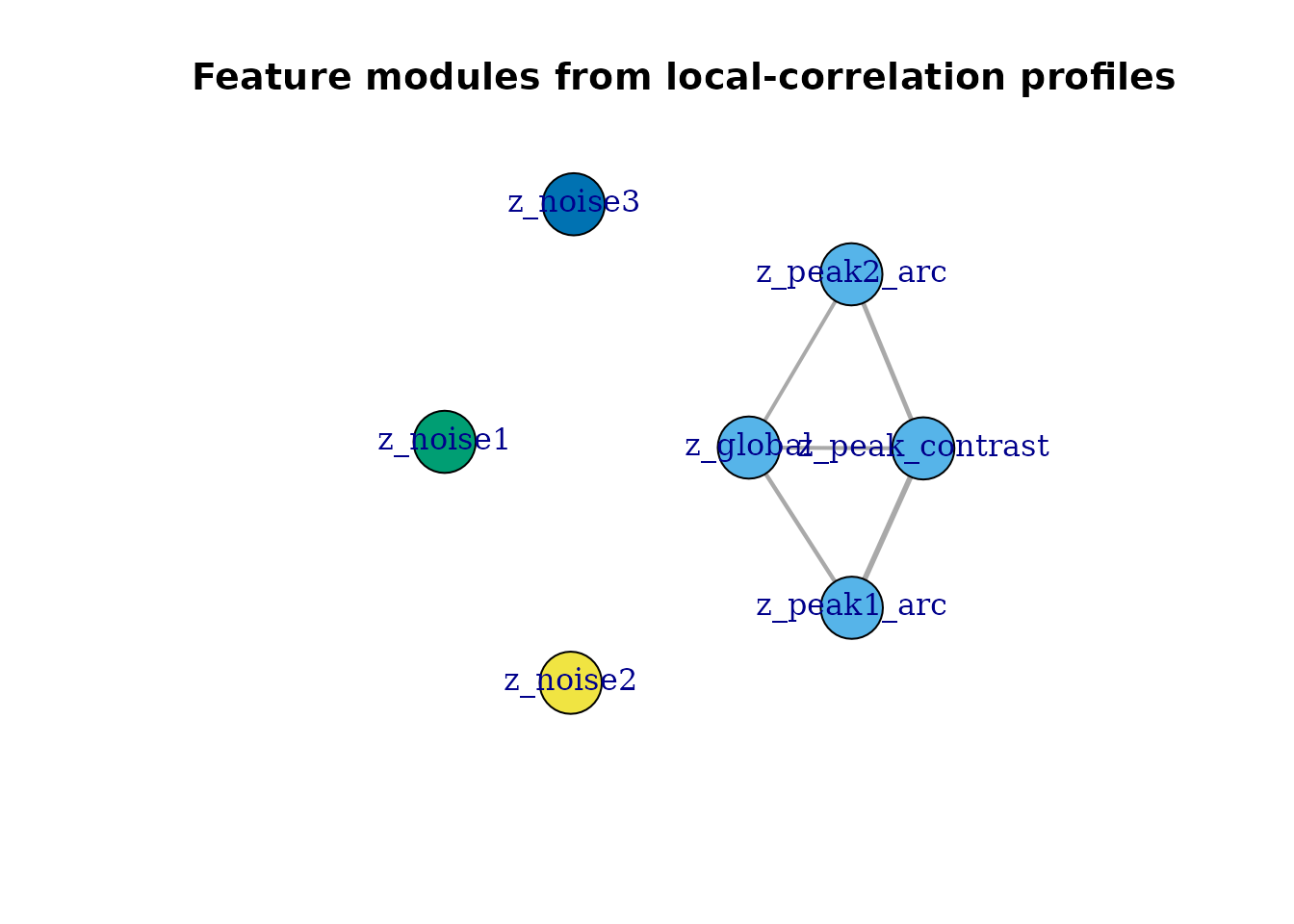
Feature modules based on similarities between local-correlation profiles. Edges pass the stated similarity threshold; they do not denote significant feature associations.
#>           feature module
#> 1        z_global      1
#> 2     z_peak1_arc      1
#> 3     z_peak2_arc      1
#> 4 z_peak_contrast      1
#> 5        z_noise1      2
#> 6        z_noise2      3
#> 7        z_noise3      4
Optional grip 3D Layout
if (requireNamespace("grip", quietly = TRUE) &&
    requireNamespace("ivue", quietly = TRUE)) {
  g <- X.graphs$geom_pruned_graphs[[k.idx]]

  X.graphs.3d <- grip::grip(
    metric = "edge_length",
    adj.list = g$adj_list,
    weight.list = g$weight_list,
    dim = 3,
    rounds = 50,
    final.rounds = 50,
    num.init = 36,
    num.nbrs = 8,
    seed = 6
  )

  ivue::plot3D.plain(X.graphs.3d, point.type = "sphere", sphere.radius = 0.03)
}
Notes
- For scientific inference, justify exchangeability and the treatment of graph selection first, then choose adequate permutation resolution and an appropriate multiple-testing procedure. More permutations do not fix an invalid null model.
- For larger datasets, use
n.cores > 1and consider chunk-level caching. - If basin refinement is unstable for a specific dataset, start with relaxed filtering and tighten thresholds gradually.