Example graphs and scalar fields
Source:vignettes/example-graphs-and-fields.Rmd
example-graphs-and-fields.RmdSmall deterministic graphs make basin definitions visible. Here we separate the graph, its edge lengths, and its scalar field, then compare selected methods under stated controls. These examples verify interfaces and illustrate structure; they do not validate performance on noisy or high-dimensional data. See Finding your way around gflow for the API catalog and the canonical workflow for all five construction families.
Recipes at a glance
| Example | Required inputs | Question and entry points | Output |
|---|---|---|---|
| Seven-vertex path | Explicit adjacency, unit lengths, two peaks including an exact plateau | How do exact level sets and terminal flow differ?
create.basin.complex(), cut()
|
Basin tables, branch hierarchy, assignments |
| Nine-vertex grid | Four-neighbor edges, unit lengths, peaks separated by level 1 | Which supports overlap? Compare trajectory flow and reachability; refine support | Membership rows and retained-support summaries |
| Two paths and an isolate | Six-vertex disconnected adjacency and field | Does the level-set hierarchy preserve components? | Three component roots with separately defined lifetimes |
| Noisy circle (linked below) | Seeded noisy coordinates, known generating field, observed response, selected dgraphs graph | How do graph choice and noise affect a basin/association analysis? | Refined basins and local-association summaries |
There are no public scientific datasets bundled in this package. The
installed extdata code manifest identifies the build; it is
not a dataset. These recipes define their inputs directly and add no
generator API or external download.
A path with two peaks and a plateau
List position is the internal vertex index. Every neighbor has a corresponding edge length in the same position, and edges appear in both directions. Field height and edge length use independent units. The drawing’s horizontal coordinate is vertex order; it is not an extra constructor input.
adjacency <- list(2L, c(1L, 3L), c(2L, 4L), c(3L, 5L),
                  c(4L, 6L), c(5L, 7L), 6L)
edge_lengths <- lapply(adjacency, function(v) rep(1, length(v)))
field <- c(0, 3, 3, 1, 2, 4, 0)
vertex_mass <- c(1, 2, 2, 1, 1, 2, 1)
vertex_density <- c(1, 1, 1, 2, 3, 2, 1)
knitr::kable(data.frame(vertex = seq_along(field), field,
                        mass = vertex_mass, density = vertex_density),
caption = "Independent field, mass, and density inputs.")| vertex | field | mass | density |
|---|---|---|---|
| 1 | 0 | 1 | 1 |
| 2 | 3 | 2 | 1 |
| 3 | 3 | 2 | 1 |
| 4 | 1 | 1 | 2 |
| 5 | 2 | 1 | 3 |
| 6 | 4 | 2 | 2 |
| 7 | 0 | 1 | 1 |
plot(seq_along(field), field, type = "b", pch = 19,
     xlab = "Vertex (unit-length path)", ylab = "Scalar field (field units)",
     ylim = c(-0.3, 4.6))
text(seq_along(field), field, labels = seq_along(field), pos = 3)
Path field: vertices 2 and 3 form one connected plateau at height 3; vertex 6 peaks at height 4. The two peaks connect through vertex 4 at height 1.
Mass expresses empirical or quadrature support. The constructor normalizes it for basin mass summaries. Density can change edge scoring in density-modulated trajectory flow; it does not weight the level-set sweep. Neither is inferred from the field. Here we use the same mass for both constructions and no density modulation, so differences arise from the basin definitions.
path_tree <- create.basin.complex(
  adjacency, edge_lengths, field, method = "superlevel_merge_tree",
  direction = "max", vertex.mass = vertex_mass
)
path_flow <- create.basin.complex(
  adjacency, edge_lengths, field, method = "trajectory_flow",
  direction = "max", vertex.mass = vertex_mass,
  method.params = list(modulation = "CLOSEST", edge.length.quantile.thld = 1)
)
stopifnot(identical(path_tree$status, "ok"),
          identical(path_flow$status, "ok"))
for (object in list(path_tree, path_flow)) {
  print(get.basin.table(object)[, c("extremum.vertex", "raw.support.size",
                                    "primary.support.size", "persistence")])
}
#>   extremum.vertex raw.support.size primary.support.size persistence
#> 1               6                7                    5           4
#> 2               2                2                    2           2
#>   extremum.vertex raw.support.size primary.support.size persistence
#> 1               2                4                    4          NA
#> 2               6                3                    3          NA
CLOSEST flow contracts the exact plateau and chooses terminal paths. Its two supports contain 4 and 3 vertices. The exact tree’s root support contains all 7 vertices, including the younger plateau branch of size 2. This hierarchical overlap is legitimate; tree support is not a partition into terminal paths.
tree <- get.basin.merge.tree(path_tree, required = TRUE)
above_two <- cut(tree, height = 2, direction = "max")
at_merge <- cut(tree, height = 1, direction = "max")
stopifnot(above_two$n.components == 2L, at_merge$n.components == 1L)
above_two$components[, c("extremum.vertex", "support.size", "vertices")]
#>   extremum.vertex support.size vertices
#> 1               2            2     2, 3
#> 2               6            2     5, 6
get.basin.assignment(path_flow)[, c("vertex", "basin.id", "next.vertex")]
#>   vertex            basin.id next.vertex
#> 1      1 basin_max_v00000002           2
#> 2      2 basin_max_v00000002          NA
#> 3      3 basin_max_v00000002           2
#> 4      4 basin_max_v00000002           3
#> 5      5 basin_max_v00000006           6
#> 6      6 basin_max_v00000006          NA
#> 7      7 basin_max_v00000006           6
At height 2, the active components are {2, 3} and
{5, 6}. At height 1 they merge. The younger branch persists
for 3 - 1 = 2 field units. The root’s finite lifetime is
4 - 0 = 4 under the component-opposite-extreme convention.
This is a structural comparison, with no significance test.
A grid with overlapping supports
Build a 3-by-3 grid with horizontal and vertical edges only. The coordinate matrix is used to construct and draw those edges. It is separate from the field and would not affect the analysis if merely redrawn.
coordinates <- as.matrix(expand.grid(x = 0:2, y = 0:2))
grid_adjacency <- lapply(seq_len(nrow(coordinates)), function(i) {
  which(rowSums(abs(sweep(coordinates, 2, coordinates[i, ], "-"))) == 1)
})
grid_lengths <- lapply(grid_adjacency, function(v) rep(1, length(v)))
grid_field <- c(0, 1, 0, 1, 3, 1, 0, 1, 2)
plot(coordinates, type = "n", asp = 1, xlab = "Graph coordinate x",
     ylab = "Graph coordinate y", xlim = c(-0.2, 2.2), ylim = c(-0.2, 2.3))
for (i in seq_along(grid_adjacency)) {
  for (j in grid_adjacency[[i]][grid_adjacency[[i]] > i]) {
    segments(coordinates[i, 1], coordinates[i, 2],
             coordinates[j, 1], coordinates[j, 2], col = "grey60")
  }
}
points(coordinates, pch = 21, bg = "white", cex = 1.5)
text(coordinates, labels = paste(seq_along(grid_field), grid_field, sep = ":"),
     pos = 3, cex = 0.9)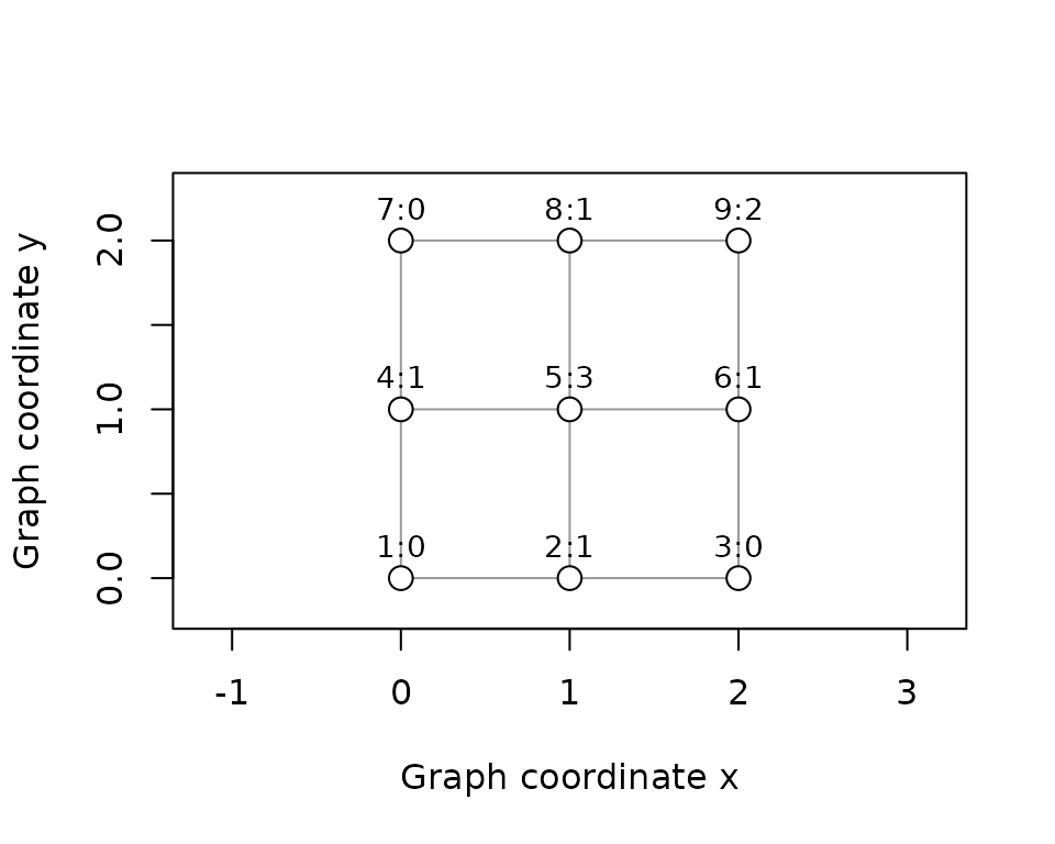
Four-neighbor grid, labeled vertex:field. The peaks at vertices 5 and 9 connect through level-1 vertices 6 and 8; diagonal shortcuts are absent.
Use all edge lengths for both methods, ascending direction, and the same explicit primary-assignment policy. No refinement is applied at first.
grid_objects <- lapply(c("trajectory_flow", "geodesic_reachability"), function(m) {
  create.basin.complex(
    grid_adjacency, grid_lengths, grid_field, method = m, direction = "max",
    method.params = list(edge.length.quantile.thld = 1,
                        primary.assignment.policy = "largest_membership_then_extremum")
  )
})
names(grid_objects) <- c("Trajectory flow", "Geodesic reachability")
stopifnot(all(vapply(grid_objects, function(x) identical(x$status, "ok"), logical(1))))
comparison <- do.call(rbind, lapply(names(grid_objects), function(method) {
  object <- grid_objects[[method]]
  membership <- get.basin.membership(object)
  data.frame(method, extrema = paste(get.basin.table(object)$extremum.vertex,
                                     collapse = ", "),
             membership.rows = nrow(membership),
             overlapping.vertices = sum(table(membership$vertex) > 1),
             uncovered.vertices = length(setdiff(seq_along(grid_field),
                                                 membership$vertex)))
}))
knitr::kable(comparison, row.names = FALSE,
             col.names = c("Method", "Peak vertices", "Membership rows",
                           "Vertices in multiple basins", "Uncovered vertices"),
caption = "Same grid and field, different basin definitions.")| Method | Peak vertices | Membership rows | Vertices in multiple basins | Uncovered vertices |
|---|---|---|---|---|
| Trajectory flow | 5, 9 | 10 | 1 | 0 |
| Geodesic reachability | 5, 9 | 13 | 4 | 0 |
get.basin.membership(grid_objects[[2]])
#>    vertex direction            basin.id membership.weight membership.status
#> 1       1       max basin_max_v00000005               1.0               raw
#> 2       2       max basin_max_v00000005               1.0               raw
#> 3       3       max basin_max_v00000005               0.5               raw
#> 4       3       max basin_max_v00000009               0.5               raw
#> 5       4       max basin_max_v00000005               1.0               raw
#> 6       5       max basin_max_v00000005               1.0               raw
#> 7       6       max basin_max_v00000005               0.5               raw
#> 8       6       max basin_max_v00000009               0.5               raw
#> 9       7       max basin_max_v00000005               0.5               raw
#> 10      7       max basin_max_v00000009               0.5               raw
#> 11      8       max basin_max_v00000005               0.5               raw
#> 12      8       max basin_max_v00000009               0.5               raw
#> 13      9       max basin_max_v00000009               1.0               raw
#>    source.stage is.primary vertex.id
#> 1  construction       TRUE         1
#> 2  construction       TRUE         2
#> 3  construction       TRUE         3
#> 4  construction      FALSE         3
#> 5  construction       TRUE         4
#> 6  construction       TRUE         5
#> 7  construction       TRUE         6
#> 8  construction      FALSE         6
#> 9  construction       TRUE         7
#> 10 construction      FALSE         7
#> 11 construction       TRUE         8
#> 12 construction      FALSE         8
#> 13 construction       TRUE         9
get.basin.assignment(grid_objects[[2]])[, c("vertex", "basin.id", "assignment.status")]
#>   vertex            basin.id assignment.status
#> 1      1 basin_max_v00000005          assigned
#> 2      2 basin_max_v00000005          assigned
#> 3      3 basin_max_v00000005          assigned
#> 4      4 basin_max_v00000005          assigned
#> 5      5 basin_max_v00000005          assigned
#> 6      6 basin_max_v00000005          assigned
#> 7      7 basin_max_v00000005          assigned
#> 8      8 basin_max_v00000005          assigned
#> 9      9 basin_max_v00000009          assigned
Both methods identify maxima 5 and 9 and cover this grid, but reachability has more overlapping vertices. A single label discards that multiplicity. Compare the membership rows first and interpret assignment as the selected policy’s convenience label. Agreement across methods is not the objective.
Draw assignments and overlapping support
These views use the same reachability result and the grid’s supplied drawing coordinates. Assignment colors show one selected label; the overlap view counts all containing basins. Neither is a probability map. Crosses indicate an absent assignment or zero support, not a third basin.
plot(grid_objects[[2]], view = "assignment", coordinates = coordinates,
     label.vertices = TRUE)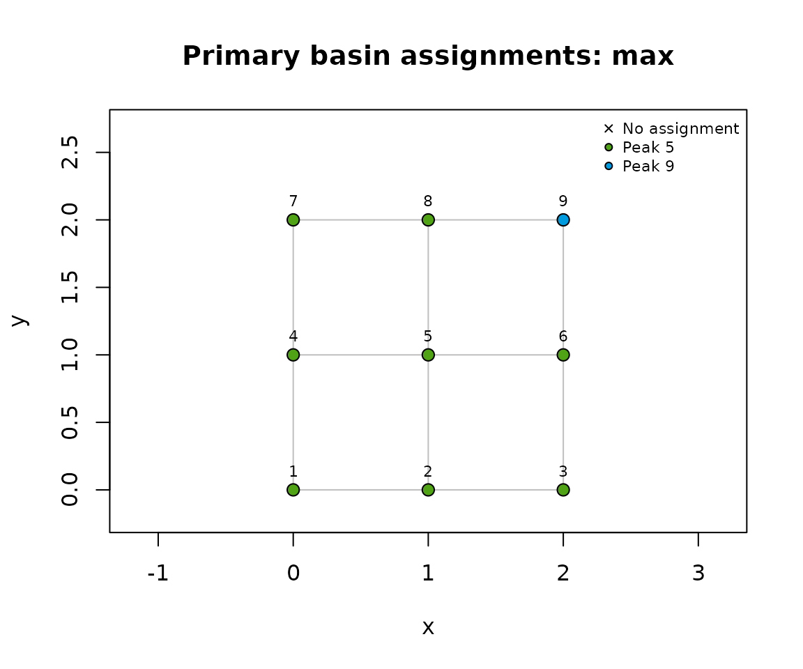
Primary reachability assignments on the grid. Colors identify the selected peak; this single label omits multiple membership.
plot(grid_objects[[2]], view = "overlap", stage = "raw",
     coordinates = coordinates, label.vertices = TRUE)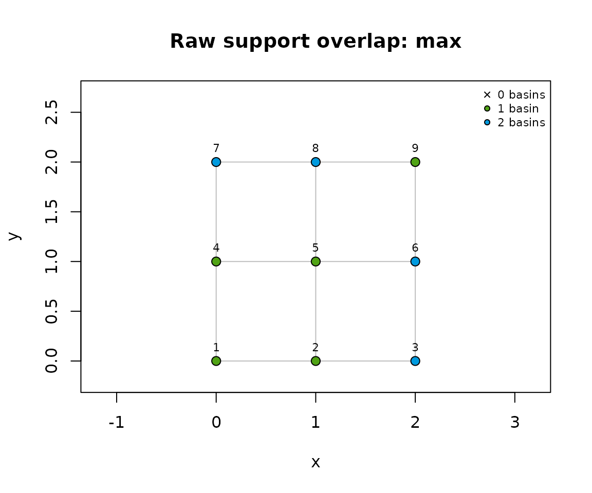
Raw reachability support counts on the same grid. Vertices in two basins retain that overlap even though the previous view selected one primary label.
Refine retained support
For reachability, retain only basins with at least six vertices. The supports initially have sizes 8 and 5, so this removes the smaller one. Expansion can then fill uncovered retained support along the graph.
refined <- create.basin.complex(
  grid_adjacency, grid_lengths, grid_field,
  method = "geodesic_reachability", direction = "max",
  method.params = list(edge.length.quantile.thld = 1,
                      primary.assignment.policy = "largest_membership_then_extremum"),
  simplify.params = list(
    support.filter = list(enabled = TRUE, min.basin.size = 6L),
    expansion = list(enabled = TRUE)
  )
)
stopifnot(identical(refined$status, "ok"))
retained <- get.basin.table(refined)
knitr::kable(retained[, c("extremum.vertex", "retained", "raw.support.size",
                         "retained.support.size")],
caption = "Refinement preserves raw support and changes retained support.")| extremum.vertex | retained | raw.support.size | retained.support.size |
|---|---|---|---|
| 5 | TRUE | 8 | 9 |
| 9 | FALSE | 5 | 0 |
raw_columns <- c("vertex", "direction", "basin.id", "membership.weight")
stopifnot(identical(get.basin.membership(refined)[, raw_columns],
                    get.basin.membership(grid_objects[[2]])[, raw_columns]))
refined$provenance$refinement.stages[, c("stage", "status")]
#>               stage    status
#> 1    relative.value  disabled
#> 2 maxima.clustering  disabled
#> 3 minima.clustering  disabled
#> 4  geometric.filter  disabled
#> 5    support.filter completed
#> 6         expansion completed
Raw membership remains a record of construction, even after retained
support changes. For current coverage, take the union of
retained.support.vertices over retained rows; for current
labels, call get.basin.assignment(refined). The canonical
workflow describes the other stages and their availability.
Disconnected components and an isolated vertex
The exact merge-tree method supports disconnected graphs. These
components are path 1--2--3, edge 4--5, and
isolated vertex 6.
disconnected_adjacency <- list(2L, c(1L, 3L), 2L, 5L, 4L, integer(0))
disconnected_lengths <- lapply(disconnected_adjacency, function(v) rep(1, length(v)))
disconnected_field <- c(0, 2, 1, 5, 4, 7)
disconnected <- create.basin.complex(
  disconnected_adjacency, disconnected_lengths, disconnected_field,
  method = "superlevel_merge_tree", direction = "max"
)
stopifnot(identical(disconnected$status, "ok"))
roots <- get.basin.table(disconnected)
stopifnot(nrow(roots) == 3L, all(is.na(roots$parent.basin.id)))
knitr::kable(roots[, c("extremum.vertex", "birth.level", "death.level", "persistence")],
caption = "Each disconnected component has its own root lifetime.")| extremum.vertex | birth.level | death.level | persistence |
|---|---|---|---|
| 6 | 7 | 7 | 0 |
| 4 | 5 | 4 | 1 |
| 2 | 2 | 0 | 2 |
No branch joins across components. The isolated vertex is a constant component with zero lifetime; its high absolute value does not give it large persistence. Mass was omitted, so mass summaries are unavailable. This example establishes component handling for exact trees, not for every trajectory backend.
From these recipes to the noisy circle
The noisy-circle vignette distinguishes latent circle position, noisy coordinates, the known generating field, and the noisy observed response. The graph is chosen from the noisy coordinates; the basin field is the observed response, not an estimated conditional mean. Its small permutation example demonstrates computation under an unrestricted row-permutation null, with assumptions and limits explained alongside it.
For a new scientific application, record which field was supplied, how the graph and lengths were chosen, the direction and method, all refinement controls, mass/density provenance, and construction status. The examples here need no optional renderer and open no browser or graphics window during builds.