Finding your way around dgraphs

dgraphs turns numerical observations into graphs and provides tools to inspect their connectivity, paths and geometry. Start with the question you want to answer. Use the task map, follow a small workflow, then consult the complete catalog.

Choose a starting point

Your question	Entry point	Choice that matters
Which nearby observations should be linked?	create.mknn.graph() or create.sknn.graph()	Mutual neighbors require agreement; symmetric neighbors accept either direction.
Can I adapt a Gabriel graph while retaining connectivity?	create.ian.graph()	Build the optional IAN backend first; inspect completion, graphs and affinity diagnostics.
How should support adapt to sampling density?	create.rknn.graph() or create.cknn.graph()	Fixed radius, local radius rules, or a geometric mean of local scales.
Should overlapping neighborhoods define edges?	create.single.iknn.graph()	Intersection graphs can connect points that are not direct nearest neighbors.
How sensitive is my graph to neighborhood size?	Plural constructors such as create.sknn.graphs()	Inspect a parameter sequence and its component counts.
Do I need paths between every pair?	graph.connected.components(), then constructor repair controls	Bridge edges make a modeling assumption across gaps.
How far apart are vertices along this graph?	graph.geodesic.distances()	Edge values must represent additive lengths or costs.
Does the graph preserve known distances?	summarize.isometry.deviation()	Requires a reference distance matrix with matching vertex order.
Do I need coordinates for a graph?	graph.embedding() or graph.spectral.embedding()	A visualization layout and a spectral representation serve different purposes.
How can I generate points with known geometry?	sample.synthetic.geometry()	Pair a geometry with a compatible sampling specification.

For powered path costs and complete-versus-restricted comparisons, read Density-sensitive paths with Fermat distances.

A first graph

Use a finite numeric matrix with observations in rows. This example samples a circle, constructs a symmetric nearest-neighbor graph, requests connectivity repair, and measures distances on the final graph.

library(dgraphs)
points <- sample.synthetic.geometry(
  synthetic.circle(),
  synthetic.sampling.grid.interval(0, 2 * pi, endpoints = "exclude.lower"),
  n = 24, seed = 17
)
X <- points$predictors
graph <- create.sknn.graph(X, k = 2, connect.components = TRUE)
print(graph)
#> Symmetric kNN graph
#> Number of vertices: 24 
#> Number of edges: 24 
#> k: 2 
#> Connected components before MST augmentation: 1 
#> Connected components after MST augmentation: 1 
#> MST bridge edges added: 0 
#> Connection method: component.mst 
#> Bridge method: none 
#> Neighbor method: exact
length(unique(graph.connected.components(graph)))
#> [1] 1
D <- graph.geodesic.distances(graph)
round(D[1:4, 1:4], 3)
#>       [,1]  [,2]  [,3]  [,4]
#> [1,] 0.000 0.261 0.522 0.783
#> [2,] 0.261 0.000 0.261 0.522
#> [3,] 0.522 0.261 0.000 0.261
#> [4,] 0.783 0.522 0.261 0.000
ig <- as_igraph(graph)
c(vertices = igraph::vcount(ig), edges = igraph::ecount(ig))
#> vertices    edges 
#>       24       24

Distances here sum straight chords between observed coordinates. They approximate circular arc distances through a finite graph; they are not exact continuous arc lengths. For a longer comparison of graph families, repair and diagnostics, read Constructing and Diagnosing Data-Derived Graphs. For sampling and embedding details, read Synthetic geometry and point sampling.

Constructing a standard graph

Use create.graph(type, ...) when you want a familiar topology or a small example. The required type selects the graph; arguments following n must be named. Every result uses the same graph accessors as a data-derived graph.

Type	Arguments	Edge lengths
"empty"	n (zero allowed)	Absent
"complete"	n	Absent
"chain"	n or x; optional span = 1, y	One, or absolute coordinate differences
"cycle"	n >= 3	Absent
"complete_bipartite"	sizes = c(n1, n2)	Absent
"star"	arms: positive edge counts along each arm	Absent
"random"	n, mean.degree; optional connected = TRUE, seed	Independent uniform lengths on [0.5, 1.5]
"circle"	n >= 3; optional sampling, edge.length, seed	Shorter unit-circle arcs (default) or chords

standard <- list(
  empty = create.graph("empty", n = 5),
  complete = create.graph("complete", n = 5),
  chain = create.graph("chain", n = 5, span = 2, labels = 101:105),
  cycle = create.graph("cycle", n = 5),
  complete_bipartite = create.graph("complete_bipartite", sizes = c(2, 3)),
  star = create.graph("star", arms = c(1, 2, 1)),
  random = create.graph("random", n = 5, mean.degree = 2, seed = 23),
  circle = create.graph("circle", n = 5, sampling = "uniform",
                        edge.length = "chord")
)
knitr::kable(data.frame(
  type = names(standard),
  vertices = vapply(standard, graph.order, integer(1)),
  edges = vapply(standard, function(g) nrow(graph.edges(g)), integer(1)),
  stored.lengths = vapply(standard, function(g) !is.null(graph.lengths(g)), logical(1))
), row.names = FALSE)

type	vertices	edges	stored.lengths
empty	5	0	FALSE
complete	5	10	FALSE
chain	5	7	TRUE
cycle	5	5	FALSE
complete_bipartite	5	6	FALSE
star	5	4	FALSE
random	5	5	TRUE
circle	5	5	TRUE

For chains, span counts positions on each side, so an interior vertex has at most 2 * span neighbors. This differs from k in nearest-neighbor workflows. Optional x sorts vertices by coordinate, with ties resolved by input position; y and labels follow the same ordering. The sorted-to-input mapping is metadata$order. An ordinary star has all arm counts equal to one; larger counts subdivide its arms.

A cycle describes topology. A circle also records unit-circle coordinates in metadata$coordinates and angles in metadata$angles. Circle sampling is "random" by default; "uniform" spaces angles equally. Choose edge.length = "chord" for Euclidean edge lengths or "arc" for shorter circular arcs. A shorter arc can cross an unsampled gap; graph shortest paths still follow the edges actually present. Arc lengths are measured in radians on the unit circle, not squared distances or conductances.

Random graphs have floor(n * mean.degree / 2) edges. A connected graph needs at least n - 1, and an impossible request errors. With connected = TRUE, a growing random tree precedes additional edges; the result is not a uniform draw from all connected graphs. With connected = FALSE, edges are sampled uniformly without replacement from all vertex pairs. Candidate storage is quadratic in the number of vertices, so this generator is intended for small examples. For both random graphs and randomly sampled circles, an explicit seed restores the caller’s random state after generation; seed = NULL uses and advances the current stream. Uniform circle sampling uses no random numbers. Unknown or irrelevant arguments error instead of being ignored.

Conventions that affect your choice

A common graph object

Every graph constructor returns a dgraph, including basic fixtures. Use graph.adjacency(graph) for its neighbor lists, graph.lengths(graph) for aligned lengths, and graph.edges(graph) for one row per undirected edge. graph.order(graph) includes isolated vertices. A bare adj.list has one integer vector per vertex, containing 1-based neighbor indices; length.list gives the corresponding finite, nonnegative lengths.

dgraph(adj.list, length.list) validates reciprocal edges and values, rejects duplicates and self-loops, and sorts neighbors and values together. Omit length.list for topology alone. A stored zero-length edge remains an edge. as_igraph(graph) preserves isolates, lengths as the length attribute, and other named edge attributes. For igraph distance calculations, explicitly use weights = igraph::E(ig)$length. Raw-list matrix conversions retain weight.list for quantities that need not represent distances.

Path-search results contain their graph in $graph and paths in $shortest.paths; a parameter sequence contains separate graph objects. Subgraphs use compact indices and record metadata$original.vertices. create.graph(type, ..., labels = ...) assigns vertex labels independently of adjacency indices. For example, labels = 101:110 names ten vertices without changing their internal indices 1:10.

Neighborhood sizes and edge quantities

All sequence constructors take an explicit, strictly increasing k.values vector with 1 <= k < n. In coordinate and graph-geodesic intersection workflows, k counts other vertices. Each cover explicitly includes its source plus those neighbors. Equal distances are resolved by vertex index, including coincident observations. Coordinate ANN search uses an exact fallback when its boundary candidates are tied. The specialized knn.metric = "linf.simplex" search currently evaluates all candidates to honor the same tie rule, with quadratic distance-evaluation cost.

X.line <- matrix(c(0, 1, 3, 6), ncol = 1)
initial <- create.single.iknn.graph(X.line, k = 1, prune.method = "none",
                                  connect.components = FALSE, verbose = FALSE)
rebuilt <- create.geodesic.iknn.graph(initial, k = 1)
rebuilt$metadata$neighborhood
#> $k
#> [1] 1
#> 
#> $effective.k
#> [1] 1 1 1 1
#> 
#> $metric
#> [1] "graph.geodesic"
#> 
#> $self
#> [1] "explicit"
#> 
#> $ties
#> [1] "distance.then.vertex.index"
#> 
#> $convention.version
#> [1] 3

Graph-geodesic construction errors if any component has fewer than k + 1 vertices. Choose small.component = "truncate" to use all reachable other vertices instead; metadata$neighborhood$effective.k records the count for each vertex, including zero for isolates. Iterated construction applies the same requested k and component policy at every rebuild.

Construction	Edge-length contract
Mutual and symmetric kNN	Euclidean distance between endpoints.
Fixed/adaptive radius and continuous kNN	Euclidean distance; radius rules govern which edges exist.
Coordinate intersection kNN	Minimum summed metric distance through a common cover member, in working coordinates after any PCA.
Geodesic intersection kNN	Previous-graph shortest-path distance between the new endpoints.
Nerve of arbitrary sets	No lengths; cardinality of overlap is the overlap edge attribute.

An overlap score or conductance is not a travel distance. Read named attributes with graph.edge.attribute(graph, "overlap"), or the corresponding column of graph.edges(graph). A length-based operation rejects a graph with no lengths; graph.geodesic.distances(graph, distance = "hop") explicitly requests unweighted distance. graph.spectrum(graph) uses the unweighted Laplacian. graph.embedding(graph) is unweighted by default; choose an edge.attribute and transform = "identity" or "reciprocal" explicitly. Layout values must be strictly positive, so zero lengths require a separate, explicit choice of layout quantity.

Connectivity, stages and cost

Mutual, symmetric and radius constructors can leave components separate. Request connect.components = TRUE when bridges are appropriate. Exact component-MST repair joins components through shortest Euclidean bridges; the ANN candidate version can fall back to exact search. A global minimum spanning tree is another repair option. join.graphs() identifies one vertex from each of two graphs and preserves aligned lengths and attributes.

graph.stages(graph) lists the stored stages. Every graph has final; constructors may additionally retain raw, pruned, raw.repaired, pruned.repaired and repaired.pruned. Pass the same stage to any accessor, as_igraph() or graph.geodesic.distances(). A missing stage errors, and stage selection never prunes, repairs or reconstructs a graph. The geodesic intersection constructor stores only final because it performs no pruning or repair. Symmetric kNN’s graph.detail = "minimal" requires both disabled.

Disconnected pairs have infinite distances. All-pairs distances require a quadratic-size matrix; request selected vertices when possible. Geometric pruning and exact component bridging can be expensive even with ANN neighbor search. Native construction is serial; thread controls do not promise native parallel execution.

Distances and stored routes

Use graph.geodesic.distances() for a matrix of distances. Supply exactly one of an existing graph or a coordinate matrix points. With coordinates, graph.type = "sknn" requires an explicit k and builds a symmetric kNN graph without pruning or connectivity repair. graph.type = "mst" builds a Euclidean minimum spanning tree and does not accept k. Setting k = 1 never changes the construction method. Coincident observations remain connected by zero-length edges when selected by the construction.

line.points <- matrix(c(0, 0, 1, 10, 11), ncol = 1)
D.tree <- graph.geodesic.distances(points = line.points, graph.type = "mst")
D.neighbors <- graph.geodesic.distances(points = line.points,
                                       graph.type = "sknn", k = 1)
knitr::kable(data.frame(
  pair = c("Coincident observations", "First to last observation"),
  tree.distance = c(D.tree[1, 2], D.tree[1, 5]),
  symmetric.neighbor.distance = c(D.neighbors[1, 2], D.neighbors[1, 5])
), row.names = FALSE, col.names = c("Pair", "Tree distance", "Symmetric kNN distance"))

Pair	Tree distance	Symmetric kNN distance
Coincident observations	0	0
First to last observation	11	Inf

Both calculations are exact shortest-path distances on their chosen graphs. Neither construction guarantees exact continuous manifold geodesics. The symmetric-neighbor example has disconnected components, represented by Inf. vertices selects matrix rows and columns in the requested order; paths may still pass through any vertex in the graph. distance = "hop" counts edges; distance = "length" requires stored lengths. To reuse a graph or choose additional construction options, construct it first and pass graph = g.

Use create.path.graph() when the routes themselves matter. Its h.values argument specifies strictly increasing positive integer maximum hop counts; a hop traverses one edge. It always returns a named collection, including when only one limit is requested. Select a member before retrieving a route.

weighted.graph <- dgraph(
  list(c(2L, 3L), c(1L, 3L, 4L), c(1L, 2L), 2L),
  list(c(5, 1), c(5, 1, 1), c(1, 1), 1))
paths <- create.path.graph(weighted.graph, h.values = c(2, 3))
knitr::kable(compare.paths(paths, from = 1, to = 4)[,
  c("h", "path_exists", "path_length", "n_hops")], row.names = FALSE,
  col.names = c("Hop limit", "Route exists", "Route length", "Hops used"))

Hop limit	Route exists	Route length	Hops used
2	TRUE	6	2
3	TRUE	3	3

get.shortest.path(paths[["h_2"]], from = 1, to = 4)
#> $path
#> [1] 1 2 4
#> 
#> $length
#> [1] 6
#> 
#> $hops
#> [1] 2
get.shortest.path(paths[["h_3"]], from = 4, to = 1)
#> $path
#> [1] 4 2 3 1
#> 
#> $length
#> [1] 3
#> 
#> $hops
#> [1] 3

With two hops, the best route has length 6; allowing three hops lowers it to 3. The returned route’s edges, stored length and hop count agree. Each result stores a graph of reachable pairs in $graph, with a hops edge attribute. get.shortest.path() returns a vertex sequence, length and hop count, or NULL when the pair is unreachable within the selected limit. Both directions are supported; a vertex’s route to itself has length and hop count zero. For equal-length routes, fewer hops are preferred. These all-pairs route collections can require substantial memory; use modest hop limits when possible.

For a path expressed as coordinates, path.length() sums Euclidean segment lengths and subdivide.path() includes both endpoints at equally spaced distances along the polyline. Points on opposite sides of a corner need not have equal straight-line distances from each other.

polyline <- rbind(c(0, 0), c(1, 0), c(1, 2))
path.length(polyline) # 3
#> [1] 3
subdivide.path(polyline, n.subdivision.pts = 5)
#>      [,1] [,2]
#> [1,] 0.00 0.00
#> [2,] 0.75 0.00
#> [3,] 1.00 0.50
#> [4,] 1.00 1.25
#> [5,] 1.00 2.00
path.dist(1:3, polyline) # normalized cumulative distances: 0, 1/3, 1
#> [1] 0.0000000 0.3333333 1.0000000

The five subdivision rows correspond to arc distances 0, 0.75, 1.5, 2.25 and 3. Repeated consecutive points contribute zero length. For a singleton or a path whose points all coincide, length and normalized cumulative distances are zero, and subdivision repeats that location. Empty paths are rejected; subdivision requires at least two output points.

Positive spectra and spectral coordinates

graph.spectrum() uses the final graph’s unweighted combinatorial Laplacian, regardless of stored lengths. Its nev counts positive eigenpairs, ordered from smallest upward. Every connected component, including an isolated vertex, contributes one omitted zero mode. The spectrum records this count as nullity and preserves component IDs in vertex order. nev = NULL requests all positive modes; use a small explicit count for large graphs. Requests larger than the number of positive modes error rather than silently changing the count.

chain <- create.graph("chain", n = 8)
spectrum <- graph.spectrum(chain, nev = 3)
round(spectrum$evalues, 6)
#> [1] 0.152241 0.585786 1.234633
spectrum$nullity
#> [1] 1
coordinates <- graph.spectral.embedding(spectrum, dim = 2)
dim(coordinates)
#> [1] 8 2

The three eigenvalues are approximately 0.152241, 0.585786 and 1.234633; the embedding uses the first two. use.R = TRUE has the same output contract. Both backends honor return.Laplacian = TRUE and return.dense; sparse output uses the optional Matrix package. The native backend uses a sparse solver for partial spectra and a dense solver for the full spectrum. The R backend uses a full dense solve, so both an R solve and a full native spectrum require quadratic memory. A documented absolute tolerance separates computed zero modes from positive modes; an unresolved separation errors explicitly.

Pass the spectrum object to graph.spectral.embedding(). Its default scale = "none" uses orthonormal eigenvectors; scale = "inverse.sqrt" scales each column by the inverse square root of its eigenvalue. With every positive mode on a connected graph, squared distances in the latter embedding equal effective resistance. With fewer modes it is a truncated representation. Neither coordinate choice generally reproduces graph shortest-path distances. Signs and bases in repeated eigenspaces can differ between solvers. Include the whole tied eigenspace when comparing distances between embeddings.

Disconnected graphs have spectra, but no common embedding is assigned: select a component with create.subgraph(graph, which(spectrum$components == id)), compute its spectrum and embed it separately. Distances between independently embedded components have no defined meaning. Empty and singleton graphs have no positive-dimensional spectral embedding.

Plotting a graph and reusing its layout

graph.embedding() computes coordinates without drawing. The standard plot() method for a dgraph computes a two-dimensional layout only when coordinates are absent and invisibly returns the coordinates actually drawn. Use vertex.values for numeric values mapped through a palette, or vertex.colors for explicit colors; supplying both errors. Constant numeric values use the palette midpoint. Every undirected edge is drawn once.

cycle <- create.graph("cycle", n = 8)
set.seed(4101)
xy <- plot(cycle, vertex.values = seq_len(8), main = "Numeric vertex values")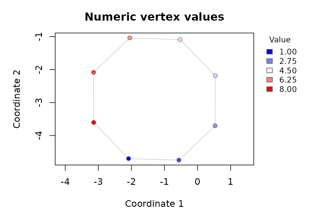

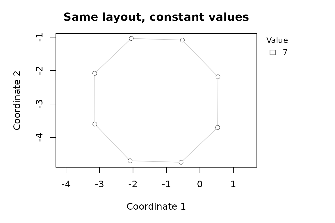
plot(cycle, coordinates = xy, vertex.values = rep(7, 8),
     main = "Same layout, constant values")

The same stage controls both layout computation and drawn edges. For three-dimensional coordinates, choose an explicit two-column projection; the plotting method never silently discards a coordinate. Layout generation itself remains available in both two and three dimensions.

set.seed(4102)
xyz <- graph.embedding(cycle, dim = 3)
colnames(xyz) <- c("x", "y", "z")
plot(cycle, coordinates = xyz, projection = c(1, 3), vertex.colors = "navy",
     main = "Explicit x/z projection")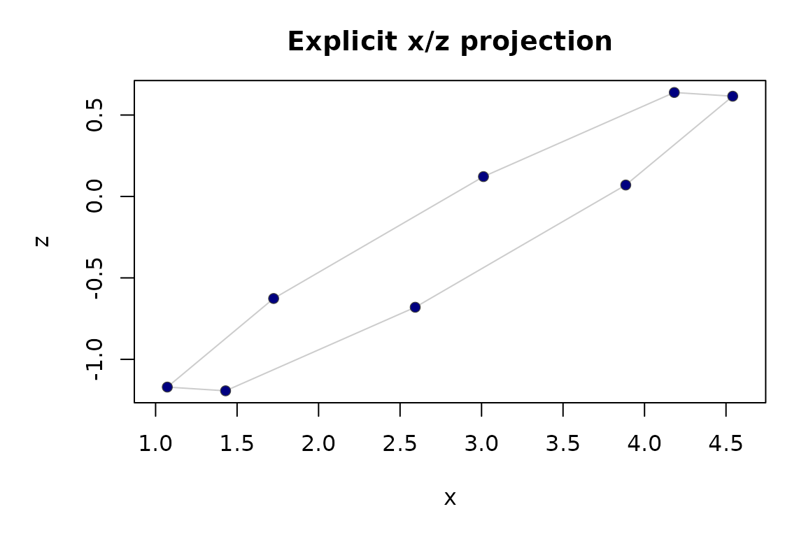

Reuse an expensive computation

Keep a constructed graph for repeated graph.geodesic.distances() calls; this reuses its edges, not a memoized distance matrix. Save D yourself when reusing the same distances. Coordinate input constructs a fresh graph for each distance call. Geodesic intersection and iterated intersection workflows deliberately build on existing graph metrics.

create.sknn.graphs() reuses one ANN search across its k values. A single symmetric constructor also accepts ordered, 1-based, non-self knn.index rows with neighbor.method = "ann"; these must correspond to the same input points. Intersection constructors expose knn.cache.path and knn.cache.mode: "read" requires a valid cache, "write" replaces it, and "readwrite" creates a missing cache but rejects an existing invalid one. Format version 3 caches store only non-self neighbors and check point values, row order, metric, working-coordinate preprocessing and maximum k. Old cache formats are rejected. The adaptive-radius sequence has a batched ANN backend. These are distinct contracts; there is no universal public neighbor-cache object shared by all constructors. Internal cache and native solver helpers are not installed public functions to call directly.

Function catalog

The catalog covers all 117 explicit public exports exactly once; 44 registered S3 methods are described separately through object workflows. Internal helpers and development applications are not public entry points. Links open the exact help included with this build, offline.

Each row is one explicit export. Open exact arguments and examples with help("create.sknn.graph", package = "dgraphs"), replacing the name as needed. The package reference manual describes the released version; newly added functions require the corresponding release or development installation.

Graph construction and parameter sequences

Function	Purpose
create.ian.graph()	Adapt local scales and prune a Gabriel graph, preserving connectivity by default; requires the optional backend.
build.ian.backend()	Build the optional pinned IAN module on macOS arm64 and return its path.
create.mknn.graph()	Build a mutual Euclidean nearest-neighbor graph, with optional pruning and repair.
create.mknn.graphs()	Build mutual-neighbor graphs across a range of neighborhood sizes.
create.sknn.graph()	Build a symmetric Euclidean nearest-neighbor graph, with optional pruning and repair.
create.sknn.graphs()	Build a symmetric-neighbor sequence using a shared ANN search.
create.rknn.graph()	Build a fixed-radius or adaptive-radius Euclidean graph.
create.rknn.graphs()	Vary the local neighborhood scale in adaptive-radius graphs.
create.cknn.graph()	Build a continuous-kNN graph using geometric-mean local scales.
create.single.iknn.graph()	Build one intersection-neighborhood graph with optional pruning.
create.iknn.graphs()	Build an intersection-neighborhood sequence and its pruning branches.
create.geodesic.iknn.graph()	Rebuild intersection neighborhoods using an existing graph’s distances.
create.iterated.iknn.graphs()	Repeat intersection construction in successive graph metrics.
build.iknn.graphs.and.selectk()	Select an intersection neighborhood size using structural or label-mixing stability.
create.cmst.graph()	Complete a Euclidean minimum spanning tree using an edge-length quantile.
create.threshold.distance.graph()	Connect points satisfying a distance threshold.
nerve.graph()	Construct a graph from overlaps between sets in a cover.

Basic graphs and representation

Function	Purpose
create.graph()	Construct standard graph types, labeled chains, random graphs and sampled circles.
dgraph()	Validate aligned neighbor, length and attribute lists as an undirected graph.
graph.adjacency()	Read the neighbor list for a stored stage.
graph.lengths()	Read aligned lengths, or NULL when absent.
graph.edges()	Read one ordered row per undirected edge, with lengths and attributes.
graph.order()	Count vertices, including isolates.
graph.stages()	List stages actually stored in a graph.
graph.edge.attribute()	Read an explicitly named edge attribute.
as_igraph()	Convert a dgraph stage to an undirected igraph object.
convert.adjacency.list.to.adjacency.matrix()	Convert bare neighbor lists to an adjacency matrix.
convert.weighted.adjacency.matrix.to.adjacency.list()	Convert a weighted adjacency matrix to aligned lists.
convert.adjacency.to.edge.matrix()	Extract an edge matrix and optional aligned weights.
count.edges()	Count undirected edges once from reciprocal neighbor lists.
compare.adj.lists()	Compare neighbor sets, optionally reporting differences.
edge.diff()	Find edges present in one graph but absent from another.
identical.vertex.set.weighted.graph.similarity()	Compare weighted graphs on the same vertex set.

Connectivity and graph editing

Function	Purpose
graph.connected.components()	Assign a component identifier to every vertex.
convert.to.undirected()	Add reciprocal links to a directed adjacency list.
rm.self.loops()	Remove each vertex from its own neighbor list.
join.graphs()	Identify one vertex from each of two graphs.
create.subgraph()	Extract the graph induced by selected vertices.
create.grid.graph()	Refine graph edges toward approximately uniform spatial spacing.

Paths and distances

Function	Purpose
fermat.knn()	Find exact complete-graph Fermat nearest neighbors.
create.fermat.sknn.graph()	Union-symmetrize exact Fermat neighbor selections.
fermat.distances()	Compute complete-graph sample Fermat distances or explicit graph-restricted alternatives.
graph.geodesic.distances()	Compute shortest-path distances for a supported graph object and stage.
compute.graph.distance()	Compute a weighted shortest-path distance between two vertices.
compute.graph.diameter()	Compute a weighted graph diameter.
get.shortest.path()	Recover a shortest vertex path.
geodesic.disk()	Find a graph neighborhood within a distance radius.
geodesic.knn()	Find nearest vertices in a graph metric.
geodesic.knnx()	Find graph-metric nearest neighbors for query vertices.
create.path.graph()	Construct a collection of path results for one or several hop limits.
create.plm.graph()	Build a path-length-matrix graph structure.
compare.paths()	Compare paths obtained under different hop limits.
minh.limit()	Find a minimum hop limit that permits a path.
path.length()	Measure Euclidean length along a coordinate path.
path.dist()	Compute normalized cumulative distance along a vertex path.
subdivide.path()	Include both endpoints and space points equally along a polyline; repeat the location for zero-length paths.

Edge lengths and pruning

Function	Purpose
extract.trajectory.edge.lengths()	Extract stored edge lengths along a graph vertex trajectory.
wgraph.prune.long.edges()	Prune edges using length constraints on alternative paths.

Diagnostics, endpoints and packing

Function	Purpose
compute.graph.summary.pmf()	Represent a degree, weight, component-size or label-neighborhood summary as probability masses.
graph.summary.divergence()	Compare graph-summary probability masses using a chosen divergence.
jensen.shannon.divergence()	Measure Jensen-Shannon divergence between probability distributions.
compute.graph.summary.stability()	Track summary divergence between consecutive graphs.
compute.stability.metrics()	Summarize structural stability of an intersection-graph sequence.
compute.geodesic.stats()	Summarize geodesic growth around grid vertices.
compute.vertex.geodesic.stats()	Inspect geodesic growth around one grid vertex.
compute.graph.endpoint.scores()	Score directional concentration in a 3D embedding using graph neighborhoods.
detect.graph.endpoints()	Select and consolidate candidate geometric endpoints.
geodesic.core.endpoints()	Detect endpoints using a graph-geodesic core.
detect.local.extrema()	Find graph-local maxima or minima of vertex values.
vertices()	Extract vertices through the generic, currently for local-extrema results.
remove.knn.outliers()	Identify and remove observations with unusual nearest-neighbor distances.
create.maximal.packing()	Select separated vertices at a requested graph scale.
validate.maximal.packing()	Check separation and maximality of a vertex packing.
verify.maximal.packing()	Verify a packing result using its graph and scale.
isometry.scale()	Fit a global scale aligning estimated distances with reference distances.
isometry.rel.rms.error()	Measure target-normalized root-mean-square distance error.
isometry.rel.abs.error()	Summarize quantiles of relative absolute distance errors.
isometry.distortion.quantiles()	Summarize multiplicative distance distortion.
isometry.distance.correlations()	Compare estimated and reference distances by correlation.
isometry.geodesic.diagnostics()	Diagnose shortcuts and distance-scale-dependent geodesic bias.
summarize.isometry.deviation()	Combine scale, error, distortion and correlation diagnostics.

Spectral methods and graph display

Function	Purpose
graph.spectrum()	Compute the smallest positive Laplacian eigenpairs, with component nullity.
graph.spectral.embedding()	Embed a connected graph from its spectrum, with explicit coordinate scaling.
graph.embedding()	Compute a graph visualization layout.

Synthetic geometry and embedding

Function	Purpose
synthetic.quadform()	Specify a flat or quadratic geometry with intrinsic and ambient dimensions.
synthetic.circle()	Specify a circle or circular arc.
synthetic.helix()	Specify a helical curve.
synthetic.trefoil()	Specify the supported trefoil parameterization.
synthetic.sphere.cap()	Specify a spherical cap over a planar footprint.
synthetic.torus.patch()	Specify a torus patch over two angular parameters.
synthetic.simplex()	Specify a compositional simplex with a given number of parts.
synthetic.stratum.point()	Specify a zero-dimensional point stratum.
synthetic.stratum.segment()	Specify a one-dimensional line-segment stratum.
synthetic.stratum.rectangle()	Specify a two-dimensional rectangular stratum.
synthetic.stratified()	Assemble compatible strata and optional junction metadata; general sampling is not implemented.
synthetic.point.line.junction()	Specify a point and segment junction.
embed.synthetic.geometry()	Deterministically map supported latent coordinates to ambient coordinates.
embed.quadform.surface()	Lift two-column coordinates using the versioned Geometry Lab quadratic arithmetic.
quadform.gradient()	Evaluate gradients of quadratic height functions.
quadform.metric()	Evaluate the induced metric of a quadratic geometry.
edge.lengths.synthetic.geometry()	Measure lifted straight latent segments; currently supports quadforms only.
validate.synthetic.geometry()	Validate a geometry specification or latent coordinate matrix.

Point sampling

Function	Purpose
sample.synthetic.geometry()	Realize geometry-only points with an explicit seed or random-state plan.
synthetic.sampling.uniform.interval()	Specify uniform interval draws and their ordering.
synthetic.sampling.grid.interval()	Specify deterministic interval points and endpoint inclusion.
synthetic.sampling.uniform.box()	Specify uniform box draws with scalar or coordinate-wise bounds.
synthetic.sampling.uniform.rectangle()	Specify two-dimensional rectangle draws.
synthetic.sampling.uniform.disk()	Specify parameter-area-uniform disk draws.
synthetic.sampling.truncated.normal()	Specify bounded normal draws on an interval.
synthetic.sampling.gapped.uniform()	Specify draws across disjoint intervals with allocation controls.
synthetic.sampling.clustered()	Specify a fixed number of two-dimensional clusters and observations per cluster.
synthetic.sampling.dirichlet.zeros()	Specify compositional draws with a fraction on a structural-zero face.
synthetic.sampling.quadform.lab()	Specify versioned quadratic-surface sampling, including surface-area rejection sampling.
validate.synthetic.sampling()	Validate a sampling specification and its compatibility with a geometry.

Interactive graph reconstruction explorer

Function	Purpose	Input and interpretation
explore.graphs()	Open the Graph Reconstruction Explorer.	A saved benchmark directory, manifest, or registered project name; optional Shiny dependencies.
read.graph.benchmark()	Read saved benchmark indexes without launching an app.	Existing dggraphui manifests and asset tables; relative paths resolve within the run.
register.graph.project()	Add a benchmark to the local project picker.	Stores a name and path; scientific assets remain outside the package.

Opening a project reads saved results without refitting. An explicit action can compute a missing weighted layout using grip and save it to a separate user cache. The default display preserves original coordinates with equal x/y/z units. A centered common-scale view preserves proportions; optional per-axis scaling is labeled as distorting proportions. Saved metric tables never change with the display.

Try the installed, deterministic twelve-point circle project:

demo <- system.file("extdata", "graph-explorer-demo", package = "dgraphs")
benchmark <- read.graph.benchmark(demo)
nrow(benchmark$graph_assets)
#> [1] 2

explore.graphs(demo)

Compare k = 2 with k = 4. The additional chords shorten graph distances relative to exact shorter unit-circle arcs. The saved GRIP layouts visualize the graphs; their apparent circularity is not the distance-error metric.

Object workflows and method help

Call a generic such as print(x), summary(x) or plot(x); R selects its registered S3 method from the object’s class. A class need not support all three operations. For example, print a symmetric graph, summarize a mutual sequence, or plot an intersection stability result. vertices(extrema) extracts vertices from detect.local.extrema() output. Geometry samples have concise print and summary methods; plot their coordinate matrices explicitly. Path-series summaries compare hop limits in a table.

The method links open version-matched help below. From R, the same topics are available through help("print.sknn_graph", package = "dgraphs"). Links inside another package’s help may require online access; dgraphs topics and their examples are included here and work without a network connection.

Generic	Object class and detailed method help
print()	dgraph; adaptive_radius_graph; build_iknn_graphs_and_selectk; cknn_graph; geodesic_stats; knn.outliers; maximal_packing; mknn_graph; mknn_graphs; mst_completion_graph; packing_validation; path.graph; path.graph.plm; radius_graph; rknn_graphs; sknn_graph; sknn_graphs; summary.knn.outliers; summary.local_extrema; summary.mst_completion_graph; synthetic_geometry_sample; summary.synthetic_geometry_sample; path.graph.series
summary()	IkNN; geodesic_stats; iknn_graphs; iterated_iknn_graphs; knn.outliers; local_extrema; mknn_graphs; mst_completion_graph; path.graph; rknn_graphs; vertex_geodesic_stats; synthetic_geometry_sample; path.graph.series
plot()	dgraph; IkNNgraphs; build_iknn_graphs_and_selectk; cst_graph_mixing_stats; geodesic_stats; iknn_stability_metrics; vertex_geodesic_stats
vertices()	local_extrema

Finding more help

help(package = "dgraphs")
help("dgraphs-package", package = "dgraphs")
vignette(package = "dgraphs")

The organization draws inspiration from the short function-purpose entries and related-help navigation in Hmisc’s overview and its usage examples. The task groups here follow dgraphs’ own API. The source repository’s make audit-guides target checks catalog completeness and method-help coverage against NAMESPACE and the maintained help sources.

Detailed help for this build

These expandable topics are generated from the installed package’s help sources. They are the same documentation opened by help() in R.

as_igraph — detailed help

Title

Convert a dgraph to igraph

Name

as_igraph

Description

Convert a dgraph to igraph

Usage

as_igraph(graph, stage = "final")

Arguments

graph	A dgraph object, including isolates.
stage	Stored graph stage.

Value

An undirected igraph. Edge lengths are named length; other attributes retain their names. No implicit weight or unit lengths are added. For metric paths pass weights = igraph::E(g)$length explicitly; for hop distance pass weights = NA.

Examples

graph <- dgraph(list(2L, 1L, integer()), list(0, 0, numeric()))
ig <- as_igraph(graph)
igraph::vcount(ig)
igraph::E(ig)$length

build.ian.backend — detailed help

Title

Build the Optional IAN Backend

Name

build.ian.backend

Description

Compile the pinned IAN and Clarabel sources installed with dgraphs in a new directory. The supported build target is macOS arm64. Setup requires Python 3, Apple’s C++ compiler/SDK, and matching native Cargo/Rust tools (Rust >= 1.77). An initial build needs cached crates or network access. No tools are installed by this function. Compilation is explicit and never starts inside create.ian.graph() or ordinary package installation.

Usage

build.ian.backend(
  build.dir,
  python = "python3",
  cargo = "cargo",
  rustc = "rustc",
  cxx = "clang++",
  offline = FALSE
)

Arguments

build.dir	New output directory, including logs and source copies. Existing files/directories are refused. A path containing spaces is allowed.
python	Python 3 command or executable path.
cargo	Cargo command or executable path from a native arm64 toolchain.
rustc	Rust compiler command or path from the same toolchain as cargo.
cxx	C++ compiler command or executable path.
offline	Logical scalar. If TRUE, Cargo uses only cached dependencies.

Value

The absolute path to dgraphs_ian.so, invisibly. Save this path and pass it to create.ian.graph(…, backend = path). Reuse the built module with the same R installation; rebuild when changing R runtime or backend sources. Build errors retain available logs and raise an R error. No shared package library is modified. Build records identify source files and tool commands.

See Also

create.ian.graph()

Examples

## Not run: 
backend <- build.ian.backend("ian-build")
fit <- create.ian.graph(matrix(c(0, 1, 2), ncol = 1), backend = backend)
stopifnot(fit$complete)

## End(Not run)

build.iknn.graphs.and.selectk — detailed help

Title

Build iKNN Graphs and Select a Neighborhood Size

Name

build.iknn.graphs.and.selectk

Description

Builds an iKNN graph sequence and selects k from structural edit-distance stability, label-mixing stability, or both.

Usage

build.iknn.graphs.and.selectk(
  X,
  k.values,
  method = c("both", "edit", "mixing", "none"),
  pca.dim = 100,
  variance.explained = 0.99,
  trim.disconnected = TRUE,
  edit.min.lcc.frac = 1,
  edit.eps = 0.05,
  labels = NULL,
  perm.blocks = NULL,
  mixing.metric = c("homophily.effect", "homophily.z", "homophily.adjusted",
    "assortativity.effect", "assortativity.z", "homophily", "assortativity",
    "conductance.median", "conductance.wmean"),
  mixing.min.lcc.frac = 0.98,
  mixing.eps = 0.05,
  mixing.require.local.extremum = TRUE,
  mixing.window = 1L,
  n.perm = 200L,
  use.edge.weights = TRUE,
  weights.are.edge.lengths = FALSE,
  affinity.method = c("exp", "inv"),
  affinity.sigma = NULL,
  affinity.sigma.from = c("k.cc.mixing", "k.max.lcc", "k.trim"),
  affinity.eps = 1e-08,
  simplify.multiple = TRUE,
  seed = 1L,
  verbose = TRUE,
  ...
)

Arguments

X	Numeric observation-by-feature matrix.
k.values	Strictly increasing integer vector of neighborhood sizes, each between 1 and n - 1.
method	Selection criterion.
pca.dim, variance.explained	PCA controls forwarded to create.iknn.graphs().
trim.disconnected	Logical; trim to a largest connected component when the requested connectivity tail is absent.
edit.min.lcc.frac, edit.eps	Connectivity and tolerance controls for edit-distance selection.
labels, perm.blocks	Optional labels and permutation blocks for mixing selection.
mixing.metric, mixing.min.lcc.frac, mixing.eps	Mixing criterion, connectivity threshold, and tolerance.
mixing.require.local.extremum, mixing.window	Local-extremum controls for the mixing curve.
n.perm	Number of label permutations.
use.edge.weights, weights.are.edge.lengths	Edge-weight interpretation.
affinity.method, affinity.sigma, affinity.sigma.from, affinity.eps	Controls for converting edge lengths to affinities.
simplify.multiple	Logical; simplify loops and multiple edges.
seed	Random seed.
verbose	Logical; report progress.
…	Additional arguments forwarded to create.iknn.graphs().

Value

An object of class “build_iknn_graphs_and_selectk” containing the graph sequence, connectivity diagnostics, selection curves, selected neighborhood sizes, trimming metadata, and call parameters.

Examples

set.seed(1)
x <- matrix(rnorm(60), ncol = 2)
selected <- build.iknn.graphs.and.selectk(x, k.values = seq.int(2, 4),
    method = "edit",
    verbose = FALSE)
selected$k.opt.edit

compare.adj.lists — detailed help

Title

Compare Two Adjacency Lists

Name

compare.adj.lists

Description

Compare Two Adjacency Lists

Usage

compare.adj.lists(adj.list1, adj.list2, verbose = FALSE)

Arguments

adj.list1	First adjacency list.
adj.list2	Second adjacency list.
verbose	Logical; print the indices of vertices with different neighbor sets. Defaults to FALSE.

Value

TRUE when each vertex has the same neighbor set in both lists, ignoring order; otherwise FALSE.

Examples

graph <- list(c(2L, 3L), 1L, 1L)
compare.adj.lists(graph, list(c(3L, 2L), 1L, 1L))

compare.paths — detailed help

Title

Compare Paths Across Hop Limits

Name

compare.paths

Description

Compare Paths Across Hop Limits

Usage

compare.paths(path.result, from, to)

Arguments

path.result	A path.graph.series object.
from	Source vertex index.
to	Target vertex index.

Value

Data frame describing path availability and length by hop limit.

Examples

graph <- list(2L, c(1L, 3L), 2L)
lengths <- list(1, c(1, 2), 2)
series <- create.path.graph(dgraph(graph, lengths), h.values = 1:2)
compare.paths(series, from = 1, to = 3)

compute.geodesic.stats — detailed help

Title

Compute Geodesic Statistics for Grid Vertices

Name

compute.geodesic.stats

Description

Analyzes how the number of geodesics scales with radius for each grid vertex. This function helps determine if collapsing/clustering geodesics is necessary and provides insights into the graph structure around grid vertices.

Usage

compute.geodesic.stats(
  adj.list,
  length.list,
  min.radius = 0.2,
  max.radius = 0.5,
  n.steps = 5,
  n.packing.vertices = length(adj.list),
  max.packing.iterations = 20,
  packing.precision = 1e-04,
  verbose = FALSE
)

Arguments

adj.list	List of integer vectors. Each vector contains indices of vertices adjacent to the corresponding vertex. Indices should be 1-based.
length.list	List of numeric vectors. Each vector contains weights of edges corresponding to adjacencies in adj.list.
min.radius	Numeric. Minimum radius as a fraction of graph diameter.
max.radius	Numeric. Maximum radius as a fraction of graph diameter.
n.steps	Integer. Number of radius steps to test.
n.packing.vertices	Integer. Number of vertices in the grid/packing.
max.packing.iterations	Integer. Maximum iterations for packing algorithm.
packing.precision	Numeric. Precision parameter for packing algorithm.
verbose	Logical. Whether to print progress information.

Value

A list of class "geodesic_stats" containing:

radii

Numeric vector. Actual radii used in the analysis.

geodesic_rays

Matrix. Number of geodesic rays for each vertex at each radius.

composite_geodesics

Matrix. Number of composite geodesics for each vertex at each radius.

path_overlap

List of matrices. Overlap statistics for each vertex at each radius.

grid_vertices

Integer vector. The vertices selected as grid vertices.

summary

Data frame. Summary statistics for each radius.

Examples

graph <- create.graph("circle", n = 8, sampling = "uniform")
stats <- compute.geodesic.stats(graph.adjacency(graph), graph.lengths(graph), min.radius = 0.3,
    max.radius = 0.5, n.steps = 2, n.packing.vertices = 4)
stats$summary

compute.graph.diameter — detailed help

Title

Compute a Weighted Graph Diameter

Name

compute.graph.diameter

Description

Compute a Weighted Graph Diameter

Usage

compute.graph.diameter(graph, stage = "final")

Arguments

graph	A dgraph with stored lengths.
stage	Stored graph stage.

Value

A list containing the diameter and the farthest path details.

Examples

graph <- list(2L, c(1L, 3L), 2L)
weights <- list(1, c(1, 2), 2)
compute.graph.diameter(dgraph(graph, weights))$diameter

compute.graph.distance — detailed help

Title

Compute a Weighted Shortest-Path Distance

Name

compute.graph.distance

Description

Compute a Weighted Shortest-Path Distance

Usage

compute.graph.distance(graph, i, j, stage = "final")

Arguments

graph	A dgraph with stored lengths.
i	Source vertex.
j	Target vertex.
stage	Stored graph stage.

Value

Numeric shortest-path distance.

Examples

graph <- list(2L, c(1L, 3L), 2L)
weights <- list(1, c(1, 2), 2)
compute.graph.distance(i = 1, j = 3, graph = dgraph(graph, weights))

compute.graph.endpoint.scores — detailed help

Title

Compute Graph Endpoint Scores from a 3D Embedding

Name

compute.graph.endpoint.scores

Description

Computes endpointness diagnostics for graph vertices by selecting graph-geodesic neighborhoods and evaluating how concentrated the corresponding 3D embedding directions are. This targets terminal arm tips in an embedding rather than graph-theoretic degree-1 vertices.

For each vertex x, let u_1, , u_m be unit vectors in the embedding from x to graph-geodesic neighbors of x. The function computes:

s_{}(x) = _{i < j} u_i^u_j

s_q(x) = {u_i^u_j : i < j}

m(x) = | _i w_i u_i |

(x) = m(x),

Neighborhoods are selected in graph-geodesic space while directions are taken from the supplied 3D embedding.

Usage

compute.graph.endpoint.scores(
  adj.list,
  length.list,
  layout.3d,
  neighborhood = c("geodesic_k", "geodesic_radius"),
  k = c(10L, 20L, 30L),
  radius = NULL,
  q = 0.1,
  neighbor.weighting = c("uniform", "inverse_distance", "gaussian"),
  gaussian.sigma = NULL,
  min.neighborhood.size = 3L,
  scale.aggregate = c("mean", "median", "min", "max"),
  verbose = FALSE
)

Arguments

adj.list	Graph adjacency list (1-based vertex indices).
length.list	Edge-length list aligned with adj.list.
layout.3d	Numeric matrix or data frame with 3 columns giving the 3D embedding coordinates for graph vertices.
neighborhood	Character string. Either “geodesic_k” (default) or “geodesic_radius”.
k	Integer vector of geodesic neighborhood sizes used when neighborhood = “geodesic_k”.
radius	Positive numeric vector of geodesic radii used when neighborhood = “geodesic_radius”.
q	Quantile used for s.q. Must lie in ⁠[0, 1]⁠. Default is 0.1.
neighbor.weighting	Character string controlling neighbor weights for m and weighted pair quantiles. One of “uniform” (default), “inverse_distance”, or “gaussian”.
gaussian.sigma	Optional positive numeric scale used when neighbor.weighting = “gaussian”. If NULL, the median positive geodesic neighborhood distance is used per vertex and scale.
min.neighborhood.size	Minimum number of usable neighbors required after removing zero-length embedding vectors. Must be at least 2.
scale.aggregate	How to aggregate scores across multiple neighborhood scales. One of “mean” (default), “median”, “min”, or “max”.
verbose	Logical; if TRUE, prints progress.

Value

A list with aggregated per-vertex scores, per-scale score matrices, and neighborhood diagnostics.

Examples

chain <- create.graph("chain", n = 8)
layout <- cbind(seq_len(8), 0, 0)
scores <- compute.graph.endpoint.scores(graph.adjacency(chain), graph.lengths(chain), layout,
    k = c(2, 3), min.neighborhood.size = 2)
head(scores$summary)

compute.graph.summary.pmf — detailed help

Title

Compute a graph summary as a probability mass function

Name

compute.graph.summary.pmf

Description

Converts a graph-like object into a named probability mass function (PMF) describing one selected graph summary. This provides a standardized bridge between graph objects and divergence functions such as jensen.shannon.divergence().

Supported v1 summaries are:

• “degree_distribution”

• “edge_weight_distribution”

• “component_size_distribution”

• “neighborhood_label_distribution”

“component_size_distribution” is included primarily as a diagnostic for disconnectedness / fragmentation, not as a general-purpose default stability summary.

Usage

compute.graph.summary.pmf(
  graph,
  summary = c("degree_distribution", "edge_weight_distribution",
    "component_size_distribution", "neighborhood_label_distribution"),
  labels = NULL,
  edge.attribute = "length",
  stage = "final",
  bins = NULL,
  n.bins = 20L,
  bin.method = c("auto", "fixed_width", "fixed_quantile", "explicit"),
  normalize = TRUE,
  support = NULL,
  zero.pad = TRUE,
  return.details = TRUE
)

Arguments

graph	A dgraph object.
summary	Summary type to compute.
labels	Optional label vector used for “neighborhood_label_distribution”. Must have length equal to the number of vertices.
edge.attribute	Edge quantity for the edge-value distribution; default “length”.
stage	Stored graph stage to summarize.
bins	Optional numeric vector of histogram breaks used for “edge_weight_distribution”.
n.bins	Integer number of bins used when bins is NULL and the summary is “edge_weight_distribution”.
bin.method	Character string controlling automatic bin construction for “edge_weight_distribution”.
normalize	Logical; if TRUE, convert counts to a PMF.
support	Optional support to align the resulting PMF to.
zero.pad	Logical; if TRUE and support is provided, missing support entries are padded with zero mass.
return.details	Logical; if TRUE, return a structured list. Otherwise return the named PMF directly.

Value

If return.details = TRUE, a list with fields:

• summary: summary type used.

• pmf: named probability mass function.

• support: support of the PMF.

• counts: named raw-count vector before normalization.

• metadata: list of summary-specific metadata.

Otherwise, returns the named PMF vector.

Examples

graph <- dgraph(list(c(2L, 3L), 1L, 1L))
compute.graph.summary.pmf(graph, summary = "degree_distribution")

compute.graph.summary.stability — detailed help

Title

Compute graph-summary stability across a graph sequence

Name

compute.graph.summary.stability

Description

Computes a divergence-based stability curve across consecutive graphs in a sequence. This function provides a generalized sequence-level analogue of the degree-profile Jensen-Shannon calculation currently used in compute.stability.metrics().

Usage

compute.graph.summary.stability(
  graphs,
  summary = c("degree_distribution", "edge_weight_distribution",
    "component_size_distribution", "neighborhood_label_distribution"),
  divergence = c("js"),
  labels = NULL,
  summary.args = list(),
  k.values = NULL,
  graph.type = c("geom", "isize"),
  return.details = TRUE
)

Arguments

graphs	Either a list of graph-like objects or an object of class “iknn_graphs”.
summary	Summary type to compare across consecutive graph pairs.
divergence	Divergence type. Currently only “js”.
labels	Optional shared vertex-label vector used for “neighborhood_label_distribution”.
summary.args	Optional named list forwarded to graph.summary.divergence().
k.values	Optional integer vector of k values. If graphs is an “iknn_graphs” object and k.values is NULL, the values are derived from its k.values attribute.
graph.type	If graphs is an “iknn_graphs” object, choose either “geom” or “isize”.
return.details	Logical; if TRUE, return a structured list.

Value

If return.details = TRUE, a list with fields:

• summary: summary type used.

• divergence: divergence type used.

• k.values: full k sequence.

• k.transition.values: k values corresponding to consecutive-graph transitions.

• values: vector of divergence values of length length(k.values) - 1.

• details: optional pairwise details for each transition.

Otherwise, returns only the divergence vector.

Examples

graphs <- list(
  dgraph(list(2L, c(1L, 3L), 2L)),
  dgraph(list(c(2L, 3L), c(1L, 3L), c(1L, 2L))),
  create.graph("complete", 3)
)
compute.graph.summary.stability(
  graphs,
  summary = "degree_distribution"
)$values

compute.stability.metrics — detailed help

Title

Compute Stability Metrics Across a Sequence of IkNN Graphs

Name

compute.stability.metrics

Description

Computes stability diagnostics across the pruned IkNN graphs produced by create.iknn.graphs(). Metrics include edit distances between consecutive graphs, graph-summary Jensen-Shannon divergence, edge-count diagnostics, local minima, and smoothed trend fits for plotting.

Usage

compute.stability.metrics(
  graphs,
  graph.type = c("geom", "isize"),
  summary = c("degree_distribution", "edge_weight_distribution",
    "component_size_distribution", "neighborhood_label_distribution"),
  divergence = c("js"),
  labels = NULL,
  summary.args = list()
)

Arguments

graphs	An object of class “iknn_graphs” returned by create.iknn.graphs().
graph.type	Character string, either “geom” or “isize”.
summary	Graph-summary family used for the divergence curve.
divergence	Divergence used for consecutive-graph comparison. Currently only “js”.
labels	Optional vertex-label vector used when summary = “neighborhood_label_distribution”.
summary.args	Optional named list forwarded to compute.graph.summary.stability().

Value

An object of class “iknn_stability_metrics”.

Examples

set.seed(1)
x <- matrix(rnorm(60), ncol = 2)
graphs <- create.iknn.graphs(x, k.values = seq.int(2, 4), compute.full = TRUE,
    verbose = FALSE)
stability <- compute.stability.metrics(graphs)
stability$edit.distances

compute.vertex.geodesic.stats — detailed help

Title

Compute Geodesic Statistics for a Single Grid Vertex

Name

compute.vertex.geodesic.stats

Description

Analyzes how the number of geodesics scales with radius for a specific grid vertex.

Usage

compute.vertex.geodesic.stats(
  adj.list,
  length.list,
  grid.vertex,
  min.radius = 0.2,
  max.radius = 0.5,
  n.steps = 5,
  n.packing.vertices = length(adj.list),
  packing.precision = 1e-04
)

Arguments

adj.list	List of integer vectors. Each vector contains indices of vertices adjacent to the corresponding vertex. Indices should be 1-based.
length.list	List of numeric vectors. Each vector contains weights of edges corresponding to adjacencies in adj.list.
grid.vertex	Integer. The grid vertex to analyze.
min.radius	Numeric. Minimum radius as a fraction of graph diameter.
max.radius	Numeric. Maximum radius as a fraction of graph diameter.
n.steps	Integer. Number of radius steps to test.
n.packing.vertices	Integer. Number of vertices in the grid/packing.
packing.precision	Numeric. Precision threshold for packing convergence.

Value

A data frame of class "vertex_geodesic_stats" with columns:

radius

Actual radius used.

rays

Number of geodesic rays within radius.

composite_geodesics

Number of composite geodesics.

overlap_min

Minimum overlap ratio.

overlap_p05

5th percentile overlap ratio.

overlap_p25

25th percentile overlap ratio.

overlap_median

Median overlap ratio.

overlap_p75

75th percentile overlap ratio.

overlap_p95

95th percentile overlap ratio.

overlap_max

Maximum overlap ratio.

Examples

graph <- create.graph("circle", n = 8, sampling = "uniform")
compute.vertex.geodesic.stats(graph.adjacency(graph), graph.lengths(graph),
    grid.vertex = 1, min.radius = 0.3,
    max.radius = 0.5, n.steps = 2)

convert.adjacency.list.to.adjacency.matrix — detailed help

Title

Convert an Adjacency List to an Adjacency Matrix

Name

convert.adjacency.list.to.adjacency.matrix

Description

Convert an Adjacency List to an Adjacency Matrix

Usage

convert.adjacency.list.to.adjacency.matrix(
  adj.list,
  weight.list = NULL,
  mode = "undirected",
  remove.self.loops = TRUE
)

Arguments

adj.list	Adjacency list.
weight.list	Optional edge-weight list aligned with adj.list.
mode	Either “undirected” or “directed”.
remove.self.loops	Logical; if TRUE, remove diagonal entries.

Value

Numeric adjacency matrix.

Examples

graph <- list(c(2L, 3L), 1L, 1L)
weights <- list(c(1, 2), 1, 2)
convert.adjacency.list.to.adjacency.matrix(graph, weights)

convert.adjacency.to.edge.matrix — detailed help

Title

Convert an Adjacency List to an Edge Matrix

Name

convert.adjacency.to.edge.matrix

Description

Convert an Adjacency List to an Edge Matrix

Usage

convert.adjacency.to.edge.matrix(adj.list, weight.list = NULL)

Arguments

adj.list	A 1-based adjacency list.
weight.list	Optional edge-weight list aligned with adj.list.

Value

A list with edge.matrix and weights.

Examples

graph <- list(c(2L, 3L), 1L, 1L)
convert.adjacency.to.edge.matrix(graph)

convert.to.undirected — detailed help

Title

Convert a Directed Adjacency List to an Undirected Adjacency List

Name

convert.to.undirected

Description

Convert a Directed Adjacency List to an Undirected Adjacency List

Usage

convert.to.undirected(adj.list)

Arguments

adj.list

Directed adjacency list.

Value

An adjacency list with reciprocal edges added and duplicate neighbors removed.

Examples

directed <- list(2L, integer(0), 1L)
convert.to.undirected(directed)

convert.weighted.adjacency.matrix.to.adjacency.list — detailed help

Title

Convert a Weighted Adjacency Matrix to Lists

Name

convert.weighted.adjacency.matrix.to.adjacency.list

Description

Convert a Weighted Adjacency Matrix to Lists

Usage

convert.weighted.adjacency.matrix.to.adjacency.list(A)

Arguments

A	Numeric square adjacency matrix.

Value

A list with adj.list and weight.list.

Examples

A <- matrix(c(0, 1, 0, 1, 0, 2, 0, 2, 0), nrow = 3)
convert.weighted.adjacency.matrix.to.adjacency.list(A)

count.edges — detailed help

Title

Count Edges in an Undirected Adjacency List

Name

count.edges

Description

Count Edges in an Undirected Adjacency List

Usage

count.edges(adj.list)

Arguments

adj.list

Adjacency list for an undirected graph.

Value

Number of undirected edges.

Examples

count.edges(list(c(2L, 3L), 1L, 1L))

create.cknn.graph — detailed help

Title

Compute a Continuous-kNN Graph

Name

create.cknn.graph

Description

Creates an undirected continuous-kNN graph using local scale distances. Let _i be the distance from observation i to its k.scale-th non-self nearest neighbor. Vertices are adjacent when

|x_i - x_j|_2 .

This is a convenience wrapper around create.rknn.graph() with type = “adaptive.radius” and radius.rule = “geomean”. It is useful as a named data-derived graph construction in geodesic reconstruction benchmarks.

Usage

create.cknn.graph(
  X,
  k.scale,
  delta = 1,
  radius.search = c("ann", "all.pairs"),
  return.timing = FALSE,
  graph.detail = c("full", "minimal"),
  prune.method = c("none", "local.geodesic", "global.geodesic.ratio"),
  max.path.edge.ratio.deviation.thld = 0.1,
  path.edge.ratio.percentile = 0.5,
  prune.tau = 1.05,
  prune.local.k = NULL,
  with.pruned.edge.stats = FALSE,
  connect.components = FALSE,
  connect.method = c("component.mst", "component.mst.ann", "global.mst"),
  bridge.k = NULL,
  bridge.k.max = NULL,
  bridge.growth = 2
)

Arguments

X	Numeric matrix or data frame with observations in rows.
k.scale	Positive integer smaller than nrow(X). Defines local scale distances _i.
delta	Positive numeric scalar multiplying the geometric-mean adaptive radius.
radius.search	Character scalar. “ann” uses the bundled ANN kd-tree exact radius-search backend inherited from create.rknn.graph(). “all.pairs” uses the direct O(n^2) reference path.
return.timing	Logical scalar. If TRUE, attach the same construction timing table returned by create.rknn.graph(), including ANN setup, local-scale search, fixed-radius candidate search, edge materialization, and graph finalization when radius.search = “ann”.
graph.detail	Character scalar. “full” returns the complete graph lifecycle object. “minimal” returns only core graph fields and is allowed only with prune.method = “none” and connect.components = FALSE.
prune.method	Character scalar. “none” disables geometric pruning. “local.geodesic” applies the experimental local geometric pruning stage before optional MST connectivity repair. “global.geodesic.ratio” applies whole-graph geodesic-ratio pruning before optional MST connectivity repair.
max.path.edge.ratio.deviation.thld	Numeric scalar in ⁠[0, 0.2)⁠. For prune.method = “global.geodesic.ratio”, an edge may be removed when the shortest alternative path is at most 1 + max.path.edge.ratio.deviation.thld times the direct edge length.
path.edge.ratio.percentile	Numeric scalar in ⁠[0, 1]⁠. For prune.method = “global.geodesic.ratio”, only edges at or above this edge length percentile are considered.
prune.tau	Numeric scalar greater than 1. For local geometric pruning, an edge may be removed when a retained local alternative path is at most this multiplicative factor times the direct edge length.
prune.local.k	Integer scalar or NULL. Number of nearest neighbors used to form local neighborhoods for pruning. For fixed-radius graphs, NULL uses the median positive raw graph degree, clipped to ⁠[1, n - 1]⁠. For adaptive-radius graphs, NULL defaults to k.scale.
with.pruned.edge.stats	Logical scalar. If TRUE, return a data frame with one row per locally pruned edge.
connect.components	Logical scalar. If TRUE, add MST bridge edges so the final graph is connected whenever possible.
connect.method	Character scalar. “component.mst” adds exact shortest inter-component bridges. “component.mst.ann” tries sparse ANN bridge candidates before automatic exact fallback. “global.mst” unions the graph with the full Euclidean MST.
bridge.k	Integer scalar or NULL. Initial ANN bridge neighborhood size for connect.method = “component.mst.ann”.
bridge.k.max	Integer scalar or NULL. Maximum ANN bridge neighborhood size before exact fallback.
bridge.growth	Numeric scalar greater than 1. Multiplicative growth factor for ANN bridge neighborhoods.

Value

A list inheriting from “cknn_graph” and “adaptive_radius_graph”. It contains the same lifecycle fields as create.rknn.graph() with type = “adaptive.radius”, radius_rule = “geomean”, radius_factor = delta, and graph_rule = “continuous.knn”.

Examples

X <- matrix(c(0, 1, 3), ncol = 1)
as.matrix(graph.edges(create.cknn.graph(X, k.scale = 1, delta = 1))[, c("from", "to")])

create.cmst.graph — detailed help

Title

Construct a Minimal Spanning Tree (MST) Completion Graph

Name

create.cmst.graph

Description

Constructs a completion of the Minimal Spanning Tree (MST) graph from a numeric data matrix. The graph is constructed in two steps: first, a MST is built connecting all data points using minimal total edge length; then, additional edges are added between any pair of points whose Euclidean distance is less than or equal to a quantile threshold based on the MST edge length distribution.

Usage

create.cmst.graph(
  X,
  q.thld = 0.9,
  pca.dim = 100,
  variance.explained = 0.99,
  verbose = TRUE
)

Arguments

X	A numeric matrix or data frame of shape n d, where each row represents a data point in d-dimensional space.
q.thld	Numeric scalar between 0 and 1 (exclusive). The quantile threshold for MST completion. Edges are added between points whose distance is less than or equal to the q.thld-quantile of MST edge weights. Default is 0.9.
pca.dim	Positive integer or NULL. If provided and ncol(X) > pca.dim, dimensionality is reduced to this many principal components before graph construction. Must be less than min(n-1, p) where n is the number of observations and p is the number of variables. Default is 100.
variance.explained	Numeric between 0 and 1 (exclusive) or NULL. If provided, selects the minimal number of PCA components such that this proportion of total variance is retained (up to pca.dim components). Ignored if pca.dim is NULL. Default is 0.99.
verbose	Logical. If TRUE, prints progress messages during computation. Default is TRUE.

Details

The MST completion process enhances connectivity in the original MST by adding edges between vertices that are "close" according to the distance distribution in the MST. This can be useful for creating more robust graph representations of data that maintain local structure while avoiding long-range connections.

When PCA is applied (either through pca.dim or variance.explained), the data is first centered and projected onto the leading principal components before graph construction. This can significantly reduce computation time for high-dimensional data while preserving the most important variation.

Value

A dgraph with raw (MST) and final (completed) stages. Use graph accessors to inspect topology and lengths; construction details are in metadata.

References

Gower, J. C., & Ross, G. J. S. (1969). Minimum spanning trees and single linkage cluster analysis. Applied Statistics, 18(1), 54-64.

See Also

stats::prcomp() for principal component analysis.

Examples

set.seed(123)
X <- matrix(rnorm(60), nrow = 20, ncol = 3)
graph <- create.cmst.graph(X, verbose = FALSE)
graph.order(graph)
nrow(graph.edges(graph))

create.geodesic.iknn.graph — detailed help

Title

Create a graph-geodesic iKNN graph

Name

create.geodesic.iknn.graph

Description

Each cover contains its source vertex plus its k nearest other vertices. Equal distances are resolved by ascending vertex index. Intersecting covers create edges whose lengths are shortest-path distances in the input graph.

Usage

create.geodesic.iknn.graph(graph, k, small.component = c("error", "truncate"))

Arguments

graph	A dgraph with stored finite, nonnegative lengths.
k	Number of nearest other vertices; integer ⁠1 <= k < n⁠.
small.component	Default “error” requires at least k + 1 vertices in every component. “truncate” uses all reachable other vertices in smaller components, recording per-vertex effective.k in neighborhood metadata.

Value

A dgraph with a final stage, lengths and an overlap edge attribute. metadata$neighborhood records requested and effective sizes and the tie rule.

Examples

graph <- create.graph("chain", 3)
create.geodesic.iknn.graph(graph, k = 1)

create.graph — detailed help

Title

Create a Standard Graph

Name

create.graph

Description

Construct a standard topology or a simple geometric graph. All types return a dgraph() and use compact, 1-based adjacency indices. type is required; type names and names in … must match exactly.

Usage

create.graph(type, n = NULL, ..., labels = NULL)

Arguments

type	Graph type: “empty”, “complete”, “chain”, “cycle”, “complete_bipartite”, “star”, “random” or “circle”.
n	Number of vertices. Required except when inferred from chain x, bipartite sizes or star arms. If supplied alongside those arguments, it must agree. Empty graphs permit zero vertices; chains require at least two, cycles and circles at least three, and other types at least one.
…	Named type-specific arguments, described below. Unknown, duplicated, unnamed and irrelevant arguments error.
labels	Optional unique, nonmissing character or numeric vertex labels, one per vertex. Labels name adjacency lists and are stored in metadata$labels; they never change adjacency indices. For chains with x, supply labels in the original input order.

Value

A dgraph with one final stage and construction information in metadata, including type. Inspect it with graph.adjacency(), graph.lengths(), graph.edges() and graph.order().

Types and arguments

empty, complete, cycle

Only n and labels. These return topology without stored lengths. A cycle closes a chain with one edge.

chain

span = 1 connects up to span positions on each side, giving at most 2 * span neighbors. It must be an integer from 1 to n - 1; it does not use the nearest-neighbor meaning of k. Optional finite numeric x orders vertices by coordinate (ties by input position) and supplies absolute coordinate differences as lengths. Without x, lengths are one. Optional vector y requires x and is reordered with it. Metadata contains order (sorted-to-input indices), x.sorted and y.sorted.

complete_bipartite

Required sizes, two positive integers. All pairs across the two parts are connected; there are no within-part edges or stored lengths. Vertices in the first part come first.

star

Required arms, at least two positive integer edge counts. Chains of those lengths share vertex 1 as their center. Thus n = 1 + sum(arms); all-one arms give an ordinary star. Vertices are numbered along successive arms. No lengths are stored.

circle

sampling = “uniform” or “random” (default), edge.length = “arc” (default) or “chord”, and optional seed. Vertices are ordered by angle on the unit circle and consecutive vertices, including last-to-first, are connected. Arc lengths measure the shorter unit-circle arc between endpoints, even when the gap in the sampling order exceeds pi. Chords are Euclidean distances. Metadata contains angles (radians) and coordinates (x/y columns).

random

Required finite mean.degree, connected = TRUE, and optional seed. The edge count is floor(n * mean.degree / 2); ⁠0 <= mean.degree <= n - 1⁠. If connected, this count must be at least n - 1. A randomly ordered growing tree is built first, then a uniform subset of remaining pairs is added. This is not uniform sampling over connected graphs or spanning trees. If disconnected graphs are allowed, a uniform subset of all pairs is sampled. Each undirected edge receives one independent length uniform between 0.5 and 1.5. Candidate-pair storage is quadratic in n; this constructor is intended for small examples. Metadata records requested and realized mean degrees and connectivity.

Random numbers

For random and circle, seed = NULL uses and advances the caller’s current random stream. An explicit nonnegative integer seed makes the call reproducible under the current RNG kind and restores the caller’s RNG state afterwards, including an initially absent state. Uniform circle sampling consumes no random numbers. The richer geometry sampling API has its own seed/state continuation contract; see sample.synthetic.geometry().

Examples

graph.order(create.graph("empty", n = 4))
graph.edges(create.graph("complete", n = 3))
chain <- create.graph("chain", x = c(3, 1, 2), span = 1,
                      labels = c("third", "first", "second"))
graph.adjacency(chain)
graph.lengths(chain)
graph.edges(create.graph("cycle", n = 4))
graph.order(create.graph("complete_bipartite", sizes = c(2, 3)))
graph.order(create.graph("star", arms = c(2, 3, 1)))
graph.edges(create.graph("random", n = 6, mean.degree = 2, seed = 10))
circle <- create.graph("circle", n = 8, sampling = "uniform",
                       edge.length = "chord")
circle$metadata$coordinates

create.grid.graph — detailed help

Title

Create a Refined Graph with Approximately Uniform Edge Spacing

Name

create.grid.graph

Description

Create a Refined Graph with Approximately Uniform Edge Spacing

Usage

create.grid.graph(
  adj.list,
  length.list,
  grid.size,
  start.vertex = 1L,
  snap.tolerance = 0.1
)

Arguments

adj.list	Input graph adjacency list.
length.list	Edge-length list matching adj.list.
grid.size	Target grid size parameter.
start.vertex	Starting vertex used for breadth-first grid placement.
snap.tolerance	Grid snapping tolerance.

Value

A dgraph object. Use graph.adjacency(), graph.lengths(), graph.edges() and graph.stages() to inspect its stored graph stages. Construction and diagnostic information is stored in metadata.

Examples

chain <- create.graph("chain", n = 3)
grid <- create.grid.graph(graph.adjacency(chain), graph.lengths(chain), grid.size = 5)
grid$metadata$grid_vertices

create.ian.graph — detailed help

Title

Construct an Iterated Adaptive Neighborhood Graph

Name

create.ian.graph

Description

Construct the initial Gabriel graph, adapt local scales and prune edges, returning graphs, affinities and diagnostics. By default, proposed bridge edges are protected so that pruning retains connectivity, and the audited retry-power numerical policy permits one checked retry after an eligible solver rejection. These are explicit variants of reference IAN.

Usage

create.ian.graph(
  X,
  distances = NULL,
  specimen.ids = NULL,
  participant.ids = NULL,
  graph = NULL,
  diagnostics = c("summary", "full"),
  backend = NULL,
  max.solves = 10000L,
  numerical.policy = "IAN evaluated-LP retry-power 0.1",
  preserve.connectivity = TRUE
)

Arguments

X	Finite numeric specimen-by-feature matrix, at least two rows and one column. There is no fixed experimental row cap. Input size must fit R/native index representations and available memory. Dense distances and affinities require quadratic storage: each n-by-n double matrix uses 8nn bytes before overhead. Several matrices/copies coexist; this is not a peak-memory estimate. Initial Gabriel construction has cubic worst-case cost. Full diagnostics retain additional dense data. See the backend guide for tested sizes.
distances	Optional unsquared distance matrix or dist. When absent, Euclidean distances are computed with stats::dist(X). Supplied distances are used exactly; duplicate feature rows must have identical distance rows. Coordinates are always required to define duplicate profiles. Row/column order must match X; named distances must match specimen IDs.
specimen.ids	Unique nonempty IDs; defaults to row names or row numbers.
participant.ids	Optional specimen-level nonempty IDs, possibly repeated.
graph	Reserved supplied-graph argument; currently must be NULL. The actual initial Gabriel graph is always constructed by IAN.
diagnostics	“summary” or “full”; full includes dense LP payloads.
backend	Optional path to the separately built dgraphs_ian.so module.
max.solves	Positive integer safety limit; reaching it returns refusal.
numerical.policy	Exactly “IAN evaluated-LP 1.0” (strict, without retries) or “IAN evaluated-LP retry-power 0.1” (default: one eligible checked retry).
preserve.connectivity	Logical scalar, default TRUE. Use FALSE for reference pruning, which may disconnect the graph. With TRUE, cache encountered bridges and skip them before testing each proposed edge’s pruning eligibility. Check noncached edges in the current graph after preceding deletions. Skips do not consume the deletion allowance. All vertices are retained. An initially disconnected graph returns refusal. This explicit variant does not change the numerical solver policy.

Details

Build the optional module once with build.ian.backend() and pass its returned path as backend. The supported build target is macOS arm64. The function itself does not compile code, download dependencies or launch an external solver. See system.file(“ian”, “README.md”, package = “dgraphs”) for the numerical contract, setup requirements and bounded qualification.

Input rows are specimens; graph vertices are unique feature profiles in first-occurrence order. Always check complete before using final_graph. Invalid R arguments or an unavailable backend raise an R error. Numerical refusal and interruption during engine execution return an incomplete result with the available diagnostics. Memory exhaustion or process termination is not a recoverable-result guarantee.

The default numerical policy is ⁠IAN evaluated-LP retry-power 0.1⁠. A rejected original return remains rejected. Its single eligible retry must itself pass strict solver success and the unchanged original-unit checks. numerical.policy=“IAN evaluated-LP 1.0” together with preserve.connectivity=FALSE selects the previous strict/reference behavior. This public default adoption changes neither policy’s implementation.

The returned top-level fields are complete, error, initial_graph, final_graph, last_valid_graph, mapping, scales, affinity, diagnostics and backend. Graphs are dgraph() objects with metric edge lengths in input distance units; affinity values are separate similarities. Mapping contains one-based representatives and member_to_profile, plus specimen, profile and participant IDs. Repeated participant IDs do not merge specimens. Error information contains kind, code and message. diagnostics$solver_history retains both accepted and rejected attempts. Backend information identifies the selected policies, source and settings. Checkpoint/resume is not exposed through this R interface.

Value

A list with complete, structured error, initial Gabriel graph, final_graph only on full completion, last_valid_graph (possibly partial), profile mapping, local scales and an affinity matrix distinct from metric edge lengths. Graph indices and mappings are one-based. Full traces retain original zero-based core indices and declare this in diagnostics. Summary diagnostics include per-solve status, acceptance, settings, residuals and iteration counts. Refusal and interruption return incomplete structured results; invalid R arguments error before native execution. Interrupts are checked at engine events; they do not interrupt an active solver call. In connectivity mode, diagnostics$connectivity contains protected.edges (one-based profile rows and IDs, first/last encounter iteration, count and first statistic), per-iteration history, and stop.reason. Iterations in this summary are one-based. Protected edges are encountered proposals, not necessarily edges that would pass the pruning criteria. Full traces also include every edge proposal and whether eligibility was tested. A complete pass with no deletion stops, including when statistical candidates remain protected. Partial results retain available protection diagnostics; final_graph remains NULL if later optimization or affinity construction fails.

See Also

build.ian.backend()

Examples

# Set this variable to the path returned by build.ian.backend().
backend <- Sys.getenv("DGRAPHS_IAN_BACKEND")
if (nzchar(backend) && file.exists(backend)) {
  X <- rbind(c(0, 0), c(1, 0), c(2, 0), c(0, 0))
  fit <- create.ian.graph(X, backend = backend,
      specimen.ids = c("alpha", "beta", "gamma", "delta"))
  stopifnot(fit$complete)
  graph.edges(fit$initial_graph)
  graph.edges(fit$final_graph)
  fit$mapping$member_to_profile # Four specimens, three unique profiles.
  fit$diagnostics$connectivity$protected.edges
}

create.iknn.graphs — detailed help

Title

Create intersection k-nearest neighbor graphs with dual pruning

Name

create.iknn.graphs

Description

For each k , builds an intersection-weighted k-NN graph and applies two pruning schemes: (1) geometric (path-to-edge ratio) and (2) intersection-size. Optionally performs PCA before graph construction.

Usage

create.iknn.graphs(
  X,
  k.values,
  max.path.edge.ratio.deviation.thld = 0.1,
  path.edge.ratio.percentile = 0.5,
  threshold.percentile = 0,
  compute.full = TRUE,
  with.isize.pruning = FALSE,
  with.edge.pruning.stats = FALSE,
  pca.dim = 100,
  variance.explained = 0.99,
  knn.metric = c("euclidean", "linf.simplex"),
  linf.tol = sqrt(.Machine$double.eps),
  verbose = TRUE,
  knn.cache.path = NULL,
  knn.cache.mode = c("none", "read", "write", "readwrite")
)

Arguments

X	A numeric matrix (or object coercible to a numeric matrix) with rows = observations and columns = features.
k.values	Strictly increasing integer vector of neighborhood sizes, each between 1 and n - 1.
max.path.edge.ratio.deviation.thld	Numeric in [0, 0.2). Geometric pruning removes an edge (i,j) when there exists an alternative path between i and j whose path/edge length ratio minus 1.0 is less than this threshold. This is a deviation threshold in [0, 0.2). Internally we compare the path-to-edge ratio R to 1 + .] or NULL. If not NULL, choose the smallest number of PCs whose cumulative variance explained exceeds this threshold, capped by pca.dim.
knn.metric	Character scalar specifying the geometry used for kNN search. “euclidean” uses ordinary ambient Euclidean distance. “linf.simplex” uses the unfolded intrinsic metric on the L^-simplex and requires rows of X to be L^-normalized.
linf.tol	Positive numeric tolerance used only when knn.metric = “linf.simplex” to identify active simplex faces and validate that max(row) = 1. Native graph construction is serial.
verbose	Logical; print progress and timing.
knn.cache.path	Optional character scalar path to a binary kNN cache file. Used only when knn.cache.mode != “none”.
knn.cache.mode	Character cache mode: “none”: always compute kNN; do not read/write cache. “read”: read kNN from cache only; if cache is missing/invalid, error. “write”: always compute kNN and atomically write/overwrite cache. “readwrite”: read valid cache when available; if cache file is missing, compute and write cache; if cache exists but is invalid, error.

Details

Geometric pruning uses the deviation threshold max.path.edge.ratio.deviation.thld and the filtering percentile path.edge.ratio.percentile. Intersection-size pruning currently uses a maximum alternative path length of 2.

Output behavior by flags:

• compute.full = FALSE: both geom_pruned_graphs and isize_pruned_graphs are NULL.

• compute.full = TRUE and with.isize.pruning = FALSE: geom_pruned_graphs is returned and isize_pruned_graphs is NULL.

Value

A list of class “iknn_graphs” with entries:

k_statistics

Matrix of per-k edge counts and reductions. (If the C++ side supplies column names, they’re preserved. Otherwise we add names consistent with what the C++ returns.)

geom_pruned_graphs

If compute.full=TRUE, list of geometrically pruned graphs (adjacency + weights); otherwise NULL.

isize_pruned_graphs

If compute.full=TRUE and with.isize.pruning=TRUE, list of intersection-size pruned graphs; otherwise NULL.

edge_pruning_stats

If with.edge.pruning.stats=TRUE, list (per k) of edge-level statistics; otherwise NULL.

Examples

# Generate sample data
X <- matrix(rnorm(100 * 5), 100, 5)

# Basic usage
res1 <- create.iknn.graphs(X, k.values = seq.int(3, 10), compute.full = FALSE)

# With custom pruning parameters
res2 <- create.iknn.graphs(X, k.values = seq.int(3, 10),
    max.path.edge.ratio.deviation.thld = 0.1,
    path.edge.ratio.percentile = 0.5, compute.full = TRUE, verbose = TRUE)

# View statistics for each k
print(res2$k_statistics)

create.iterated.iknn.graphs — detailed help

Title

Create iterated graph-geodesic iKNN graphs

Name

create.iterated.iknn.graphs

Description

Constructs G0 with create.iknn.graphs(), then constructs G1, G2, …, Gm by repeatedly applying create.geodesic.iknn.graph() to each graph in the k.values sequence. This implements the iterated nerve rule

{i,j} E(G_{t+1}) kNN_{G_t}(i) kNN_{G_t}(j) ,

with edge length

{t+1}(i,j) = d{G_t}(i,j).

Usage

create.iterated.iknn.graphs(
  X,
  k.values,
  n.iterations = 3L,
  small.component = c("error", "truncate"),
  max.path.edge.ratio.deviation.thld = 0,
  path.edge.ratio.percentile = 0.5,
  threshold.percentile = 0,
  pca.dim = 100,
  variance.explained = 0.99,
  verbose = TRUE,
  knn.cache.path = NULL,
  knn.cache.mode = c("none", "read", "write", "readwrite")
)

Arguments

X	Numeric matrix with rows as observations and columns as features.
k.values	Strictly increasing integer vector of neighborhood sizes, each between 1 and n - 1.
n.iterations	Non-negative integer number of geodesic rebuilds after G0. The default 3 returns G0, G1, G2, and G3.
small.component	Component-size policy forwarded to every geodesic rebuild.
max.path.edge.ratio.deviation.thld, path.edge.ratio.percentile, threshold.percentile	Initial G0 pruning arguments forwarded to create.iknn.graphs(). The default deviation and quantile thresholds are zero so that G0 is the unpruned iKNN 1-skeleton.
pca.dim, variance.explained, verbose, knn.cache.path, knn.cache.mode	Additional arguments forwarded to create.iknn.graphs() for the initial G0 construction.

Value

A list of class “iterated_iknn_graphs” with entries:

k.values

Integer vector of requested k values.

n_iterations

Number of geodesic rebuilds after G0.

initial_graphs

The “iknn_graphs” object returned by create.iknn.graphs() for G0.

graphs

Nested list named G0, G1, …; each entry is a named list of graph objects for k.values.

summary

Data frame with one row per iteration and k.

Examples

set.seed(1)
X <- matrix(rnorm(30), ncol = 2)
out <- create.iterated.iknn.graphs(X, k.values = seq.int(2, 3), n.iterations = 1,
    verbose = FALSE)
out$summary

create.maximal.packing — detailed help

Title

Create a Maximal Packing of Vertices in a Graph

Name

create.maximal.packing

Description

Creates a maximal packing of vertices based on a specified grid size. The algorithm places vertices in the graph using a separation distance that produces a vertex set packing of size approximately equal to the given grid size. A vertex packing is a set of vertices where each pair is separated by at least a specified distance.

Usage

create.maximal.packing(
  adj.list,
  length.list,
  grid.size,
  max.iterations = 20,
  precision = 0.1
)

Arguments

adj.list	A list where each element is a vector of adjacent vertex indices (1-based) for the corresponding vertex. Must represent an undirected graph.
length.list	A list where each element is a vector of edge weights corresponding to the adjacencies in adj.list. All weights must be positive.
grid.size	A positive integer (>= 2) specifying the approximate separation distance between vertices in the packing.
max.iterations	Maximum number of iterations for the algorithm to converge. Default is 20.
precision	Precision threshold for convergence of the algorithm. Must be between 0 and 0.5. Default is 0.1.

Details

The function computes a maximal packing by iteratively selecting vertices that are approximately grid.size apart from each other. The process starts from one of the graph’s diameter endpoints (determined automatically) and continues until no more vertices can be added to the packing without violating the distance constraint.

The returned \code{graph_diameter} represents the longest shortest path
in the graph, which provides insight into the graph's overall structure
and extent.

The \code{max_packing_radius} value indicates the minimum distance that
separates any two vertices in the packing. This value is determined
through binary search to achieve a packing of approximately the
requested size.

The function validates input parameters and ensures that the graph
structure is properly specified before computing the packing. The graph
must be undirected (symmetric adjacency) and connected.

Value

A maximal_packing result containing its graph (a dgraph), grid_vertices (packing indices), graph_diameter, and max_packing_radius (the guaranteed separation of packing vertices).

See Also

validate.maximal.packing, verify.maximal.packing

Examples

adj.list <- list(c(2), c(1, 3), c(2, 4), c(3, 5), c(4))
length.list <- list(c(1), c(1, 1), c(1, 1), c(1, 1), c(1))

result <- create.maximal.packing(adj.list, length.list, grid.size = 2)
result$grid_vertices
result$max_packing_radius

create.mknn.graph — detailed help

Title

Compute a Mutual k-Nearest Neighbor Graph with Weights

Name

create.mknn.graph

Description

Creates an undirected graph where two points are connected by an edge if and only if they are present in each other’s k-nearest neighbor (kNN) lists. The weight of each edge represents the distance between the connected vertices.

Usage

create.mknn.graph(
  X,
  k,
  prune.method = c("none", "local.geodesic", "global.geodesic.ratio"),
  max.path.edge.ratio.deviation.thld = 0.1,
  path.edge.ratio.percentile = 0.5,
  prune.tau = 1.05,
  prune.local.k = NULL,
  with.pruned.edge.stats = FALSE,
  connect.components = FALSE,
  connect.method = c("component.mst", "component.mst.ann", "global.mst"),
  bridge.k = NULL,
  bridge.k.max = NULL,
  bridge.growth = 2
)

Arguments

X	A numeric matrix or data frame where each row represents a data point and each column represents a feature/dimension.
k	A positive integer specifying the number of nearest neighbors to consider, excluding self; require ⁠1 <= k < n⁠.
prune.method	Character scalar. “none” disables geometric pruning. “local.geodesic” applies the experimental local geometric pruning stage before optional MST connectivity repair. “global.geodesic.ratio” applies whole-graph geodesic-ratio pruning before optional MST connectivity repair.
max.path.edge.ratio.deviation.thld	Numeric scalar in ⁠[0, 0.2)⁠. For prune.method = “global.geodesic.ratio”, an edge may be removed when the shortest alternative path is at most 1 + max.path.edge.ratio.deviation.thld times the direct edge length.
path.edge.ratio.percentile	Numeric scalar in ⁠[0, 1]⁠. For prune.method = “global.geodesic.ratio”, only edges at or above this edge length percentile are considered.
prune.tau	Numeric scalar greater than 1. For local geometric pruning, an edge may be removed when a retained local alternative path is at most this multiplicative factor times the direct edge length.
prune.local.k	Integer scalar or NULL. Number of nearest neighbors used to form local neighborhoods for pruning. Defaults to k.
with.pruned.edge.stats	Logical scalar. If TRUE, return a data frame with one row per locally pruned edge.
connect.components	Logical scalar. If TRUE, add MST bridge edges so the final graph is connected whenever possible.
connect.method	Character scalar. “component.mst” adds exact shortest inter-component bridges. “component.mst.ann” tries sparse ANN bridge candidates before automatic exact fallback. “global.mst” unions the graph with the full Euclidean MST.
bridge.k	Integer scalar or NULL. Initial ANN bridge neighborhood size for connect.method = “component.mst.ann”.
bridge.k.max	Integer scalar or NULL. Maximum ANN bridge neighborhood size before exact fallback.
bridge.growth	Numeric scalar greater than 1. Multiplicative growth factor for ANN bridge neighborhoods.

Details

The mutual k-nearest neighbor graph is a symmetric graph where an edge between vertices i and j exists if and only if:

• j is among the k nearest neighbors of i, AND

• i is among the k nearest neighbors of j

This mutual relationship ensures that the resulting graph is undirected and typically sparser than a standard k-nearest neighbor graph.

Use graph accessors for the final graph and graph.stages() to list stored raw, pruned and repaired stages. Construction details are in metadata.

Value

A dgraph object. Use graph.adjacency(), graph.lengths(), graph.edges() and graph.stages() to inspect its stored graph stages. Construction and diagnostic information is stored in metadata.

See Also

create.mknn.graphs for creating multiple graphs with different k values, summary.mknn_graphs for summarizing graph properties

Examples

set.seed(123)
X <- matrix(rnorm(60), ncol = 2)
graph <- create.mknn.graph(X, k = 4)
graph.order(graph)
nrow(graph.edges(graph))
graph.adjacency(graph)[[1]]

create.mknn.graphs — detailed help

Title

Create Multiple Mutual kNN Graphs with Geometric Pruning

Name

create.mknn.graphs

Description

Constructs a series of mutual k-nearest neighbor (MkNN) graphs across a range of k values, with optional geometric pruning to remove redundant edges based on alternative path analysis.

Usage

create.mknn.graphs(
  X,
  k.values,
  max.path.edge.ratio.thld = 1.2,
  path.edge.ratio.percentile = 0.5,
  compute.full = FALSE,
  pca.dim = 100,
  variance.explained = 0.99,
  verbose = FALSE
)

Arguments

X	A numeric matrix where rows represent data points and columns represent features. Data frames will be converted to matrices.
k.values	Strictly increasing integer vector of neighborhood sizes, each between 1 and n - 1.
max.path.edge.ratio.thld	Maximum acceptable ratio of alternative path length to direct edge length for pruning; zero disables pruning. Edges with alternative paths having ratio <= this value will be pruned. Default is 1.2. Set to 0 to disable pruning.
path.edge.ratio.percentile	Percentile threshold (0.0-1.0) for edge lengths to consider for pruning. Only edges with length greater than this percentile are evaluated. Default is 0.5.
compute.full	Logical; if TRUE, returns complete graph structures for each k value. If FALSE, returns only summary statistics. Default is FALSE.
pca.dim	Maximum number of principal components to use if dimensionality reduction is applied. Default is 100. Set to NULL to skip dimensionality reduction.
variance.explained	Target percentage of variance to be explained by the principal components (0-1). Default is 0.99. If this can be achieved with fewer than pca.dim components, the smaller number is used. Set to NULL to use exactly pca.dim components.
verbose	Logical; if TRUE, displays progress messages. Default is FALSE.

Details

This function performs the following steps for each k value:

1. Mutual kNN Graph Construction: Creates a graph where edges exist only between mutually nearest neighbors.

2. Geometric Pruning (optional): Removes edges where alternative paths exist with acceptable length ratios. An edge (i,j) is pruned if there exists a path i->k->j such that (d(i,k) + d(k,j)) / d(i,j) <= threshold.

3. Dimensionality Reduction (optional): If the data has more than pca.dim dimensions, PCA is applied before graph construction to improve computational efficiency and reduce noise.

The geometric pruning step helps create sparser graphs by removing edges that can be well-approximated by two-hop paths, which can improve graph quality for clustering and visualization tasks.

Value

An object of class "mknn_graphs" containing:

k_statistics

A data frame with columns: k (k value), n_edges (edges before pruning), n_edges_pruned (edges after pruning), n_removed (number of removed edges), reduction_ratio (proportion of edges removed).

pruned_graphs

If compute.full=TRUE, a named list of pruned graphs for each k value. NULL otherwise.

edge_pruning_stats

A list of pruning statistics for each k value, containing edge lengths and path ratios.

The returned object also has the following attributes:

• k.values: The requested neighborhood sizes

• max.path.edge.ratio.thld: The pruning threshold used

• path.edge.ratio.percentile: The percentile threshold used

• pca: If PCA was performed, contains dimensionality reduction details

See Also

create.mknn.graph for creating a single MkNN graph, summary.mknn_graphs for summarizing the results

Examples

set.seed(123)
X <- matrix(rnorm(80), ncol = 2)
result <- create.mknn.graphs(X, k.values = seq.int(3, 4), compute.full = TRUE, verbose = FALSE)
result$k_statistics

X.high <- matrix(rnorm(120), nrow = 20, ncol = 6)
result.pca <- create.mknn.graphs(X.high, k.values = seq.int(2, 3), pca.dim = 3, verbose = FALSE)
attr(result.pca, "pca")$n_components

create.path.graph — detailed help

Title

Construct Path Graphs Across Hop Limits

Name

create.path.graph

Description

Find minimum-length routes using at most each requested number of edges. Equal-length routes prefer fewer hops. One route is stored per unordered pair and can be retrieved in either direction with get.shortest.path().

Usage

create.path.graph(graph, h.values, stage = "final")

Arguments

graph	A dgraph with finite nonnegative stored lengths.
h.values	One or more strictly increasing positive integer hop limits. A hop counts one traversed edge. Invalid, duplicate or unordered values error; values are never silently rounded or reordered.
stage	Stored graph stage; defaults to “final”.

Details

Hop-constrained search retains a separate distance for each hop count, then selects the best route for each pair. With nonnegative lengths, limits above n - 1 need no additional search. For each source, auxiliary storage is proportional to n * min(h, n - 1); storing routes for all reachable pairs can require cubic space. Use small hop limits when possible.

Value

A named path.graph.series collection, even for one limit. Names are h_2, h_4, etc. Each member is a path.graph with a graph of reachable pairs, stored shortest.paths, and an h attribute recording the requested limit. Its graph stores route lengths and a hops edge attribute. Routes use the input graph’s vertex indices. Empty graphs and isolated vertices are preserved.

Examples

graph <- create.graph("chain", n = 5)
paths <- create.path.graph(graph, h.values = c(2, 4))
get.shortest.path(paths[["h_4"]], from = 1, to = 5)
get.shortest.path(paths[["h_4"]], from = 5, to = 1)
compare.paths(paths, from = 1, to = 5)

create.plm.graph — detailed help

Title

Create a Path Length Matrix Graph Structure

Name

create.plm.graph

Description

Create a Path Length Matrix Graph Structure

Usage

create.plm.graph(adj.list, length.list, h)

Arguments

adj.list	Adjacency list using 1-based vertex indices.
length.list	Edge-length list matching adj.list.
h	Odd positive integer maximum path length in hops.

Value

An object of class path.graph.plm.

Examples

graph <- list(2L, c(1L, 3L), 2L)
lengths <- list(1, c(1, 2), 2)
create.plm.graph(graph, lengths, h = 3)

create.rknn.graph — detailed help

Title

Compute a Radius-kNN Graph

Name

create.rknn.graph

Description

Creates an undirected Euclidean radius graph from a numeric data matrix. Use type = “fixed” for a fixed-radius graph, where vertices i and j are adjacent exactly when their Euclidean distance is at most radius. Use type = “adaptive.radius” for an adaptive-radius graph based on observation-specific local scale distances.

Usage

create.rknn.graph(
  X,
  type = c("fixed", "adaptive.radius"),
  radius = NULL,
  k.scale = NULL,
  radius.factor = 1,
  radius.rule = c("max", "min", "geomean"),
  radius.search = c("ann", "all.pairs"),
  return.timing = FALSE,
  graph.detail = c("full", "minimal"),
  prune.method = c("none", "local.geodesic", "global.geodesic.ratio"),
  max.path.edge.ratio.deviation.thld = 0.1,
  path.edge.ratio.percentile = 0.5,
  prune.tau = 1.05,
  prune.local.k = NULL,
  with.pruned.edge.stats = FALSE,
  connect.components = FALSE,
  connect.method = c("component.mst", "component.mst.ann", "global.mst"),
  bridge.k = NULL,
  bridge.k.max = NULL,
  bridge.growth = 2
)

Arguments

X	Numeric matrix or data frame with observations in rows.
type	Character scalar. “fixed” builds a fixed-radius graph using radius. “adaptive.radius” builds an adaptive-radius graph using k.scale, radius.factor, and radius.rule.
radius	Positive numeric scalar. Edges are included when |x_i - x_j|_2 radius. Required for type = “fixed”.
k.scale	Positive integer smaller than nrow(X). Defines local scale distances _i. Required for type = “adaptive.radius”.
radius.factor	Positive numeric scalar multiplying the adaptive radius.
radius.rule	Character scalar. “max” uses d_{ij} radius.factor (_i,j); “min” uses d{ij} radius.factor (_i,j); and “geomean” uses d{ij} radius.factor . The “geomean” rule is the continuous-kNN support rule.
radius.search	Character scalar. “ann” uses the bundled ANN kd-tree to perform exact fixed-radius candidate searches before applying the pair-specific adaptive-radius rule. “all.pairs” uses the direct O(n^2) pair scan and is retained as a reference path. Used only for type = “adaptive.radius”.
return.timing	Logical scalar. If TRUE, attach a construction timing table for adaptive-radius graphs.
graph.detail	Character scalar. “full” returns the complete graph lifecycle object for adaptive-radius graphs. “minimal” returns only the graph fields needed by fitting code and is currently allowed only for adaptive-radius graphs with prune.method = “none” and connect.components = FALSE.
prune.method	Character scalar. “none” disables geometric pruning. “local.geodesic” applies the experimental local geometric pruning stage before optional MST connectivity repair. “global.geodesic.ratio” applies whole-graph geodesic-ratio pruning before optional MST connectivity repair.
max.path.edge.ratio.deviation.thld	Numeric scalar in ⁠[0, 0.2)⁠. For prune.method = “global.geodesic.ratio”, an edge may be removed when the shortest alternative path is at most 1 + max.path.edge.ratio.deviation.thld times the direct edge length.
path.edge.ratio.percentile	Numeric scalar in ⁠[0, 1]⁠. For prune.method = “global.geodesic.ratio”, only edges at or above this edge length percentile are considered.
prune.tau	Numeric scalar greater than 1. For local geometric pruning, an edge may be removed when a retained local alternative path is at most this multiplicative factor times the direct edge length.
prune.local.k	Integer scalar or NULL. Number of nearest neighbors used to form local neighborhoods for pruning. For fixed-radius graphs, NULL uses the median positive raw graph degree, clipped to ⁠[1, n - 1]⁠. For adaptive-radius graphs, NULL defaults to k.scale.
with.pruned.edge.stats	Logical scalar. If TRUE, return a data frame with one row per locally pruned edge.
connect.components	Logical scalar. If TRUE, add MST bridge edges so the final graph is connected whenever possible.
connect.method	Character scalar. “component.mst” adds exact shortest inter-component bridges. “component.mst.ann” tries sparse ANN bridge candidates before automatic exact fallback. “global.mst” unions the graph with the full Euclidean MST.
bridge.k	Integer scalar or NULL. Initial ANN bridge neighborhood size for connect.method = “component.mst.ann”.
bridge.k.max	Integer scalar or NULL. Maximum ANN bridge neighborhood size before exact fallback.
bridge.growth	Numeric scalar greater than 1. Multiplicative growth factor for ANN bridge neighborhoods.

Value

A dgraph, with constructor class radius_graph for fixed radii or adaptive_radius_graph for adaptive radii. Use graph accessors for topology, lengths and retained stages; construction diagnostics are in metadata.

Examples

X <- matrix(c(0, 1, 3), ncol = 1)
as.matrix(graph.edges(create.rknn.graph(X, type = "fixed", radius = 1.1))[, c("from", "to")])
as.matrix(graph.edges(create.rknn.graph(X, type = "adaptive.radius", k.scale = 1))[, c("from",
"to")])

create.rknn.graphs — detailed help

Title

Compute Adaptive Radius-kNN Graphs Across k Values

Name

create.rknn.graphs

Description

Creates a sequence of adaptive-radius graphs by varying the k.scale parameter passed to create.rknn.graph(type = “adaptive.radius”). By default, ANN-backed construction uses the batched C++ backend while the direct all-pairs reference path uses the scalar R loop. Set backend = “r” to force the scalar loop for ANN parity checks.

Usage

create.rknn.graphs(X, k.values, ..., backend = c("auto", "cpp", "r"))

Arguments

X	Numeric matrix or data frame with observations in rows.
k.values	Strictly increasing integer vector, each between 1 and n - 1. Returned graphs follow this order.
…	Additional arguments forwarded to create.rknn.graph() with type = “adaptive.radius”. The arguments type, k.scale, and radius are reserved by this plural constructor.
backend	Character scalar. “auto” uses the batched C++ ANN backend when radius.search = “ann” and the scalar R loop when radius.search = “all.pairs”. “cpp” forces the batched C++ ANN backend and therefore requires radius.search = “ann”. “r” forces the scalar R loop and is retained as a reference parity backend.

Value

A list of class “rknn_graphs” with components:

graphs

A named list of adaptive-radius graph objects, one per k.

k_statistics

A data frame with one row per k containing edge, component, and MST-repair counts.

timing

Present only when forwarded options request graph timing; contains backend-specific construction timing rows.

Attributes include k.values and n_vertices.

See Also

create.rknn.graph()

Examples

X <- matrix(c(0, 1, 3, 4), ncol = 1)
result <- create.rknn.graphs(X, k.values = seq.int(1, 2), radius.search = "all.pairs",
    graph.detail = "minimal",
    prune.method = "none")
names(result$graphs)
result$k_statistics

create.single.iknn.graph — detailed help

Title

Create a Single Intersection-weighted k-Nearest Neighbors Graph

Name

create.single.iknn.graph

Description

Creates and prunes an intersection-weighted k-nearest neighbors (IWD-kNN) graph from input data. The graph is constructed based on feature space distances and intersection sizes between neighbor sets.

Usage

create.single.iknn.graph(
  X,
  k,
  max.path.edge.ratio.deviation.thld = 0.1,
  prune.method = c("global.geodesic", "none", "local.geodesic", "global.geodesic.ratio"),
  prune.tau = NULL,
  prune.local.k = NULL,
  path.edge.ratio.percentile = 0.5,
  threshold.percentile = 0,
  compute.full = FALSE,
  with.isize.pruning = FALSE,
  with.edge.pruning.stats = FALSE,
  pca.dim = 100,
  variance.explained = 0.99,
  knn.metric = c("euclidean", "linf.simplex"),
  linf.tol = sqrt(.Machine$double.eps),
  connect.components = FALSE,
  connect.method = c("component.mst", "component.mst.ann", "global.mst"),
  bridge.k = NULL,
  bridge.k.max = NULL,
  bridge.growth = 2,
  with.lifecycle.branches = FALSE,
  verbose = TRUE,
  knn.cache.path = NULL,
  knn.cache.mode = c("none", "read", "write", "readwrite")
)

Arguments

X	A numeric matrix where rows represent data points and columns represent features. Data frames will be coerced to matrices.
k	Integer scalar. Number of nearest other vertices. Self is explicitly added to each cover, and distance ties use ascending vertex index. Must be positive and less than the number of data points.
max.path.edge.ratio.deviation.thld	Numeric in [0, 0.2). Geometric pruning removes an edge (i,j) when there exists an alternative path between i and j whose path/edge length ratio minus 1.0 is less than this threshold. This is a deviation threshold in [0, 0.2). Internally we compare the path-to-edge ratio R to 1 + . Used when prune.method is “global.geodesic” or “global.geodesic.ratio”.
prune.method	Character scalar. “global.geodesic” preserves the historical whole-graph geometric pruning behavior controlled by max.path.edge.ratio.deviation.thld and path.edge.ratio.percentile. “global.geodesic.ratio” is a separately named alias for that whole-graph geodesic-ratio behavior. “local.geodesic” applies the same experimental local geometric pruning stage used by sKNN/mKNN. “none” disables geometric pruning; quantile pruning controlled by threshold.percentile is still honored.
prune.tau	Numeric scalar greater than 1, or NULL. Multiplicative threshold for local geometric pruning. If NULL, defaults to max(1 + max.path.edge.ratio.deviation.thld, 1.05).
prune.local.k	Integer scalar or NULL. Number of nearest neighbors used to form local neighborhoods for local geometric pruning. Defaults to k.
path.edge.ratio.percentile	Numeric in [0,1]. Only edges with length above this percentile are considered for geometric pruning.
threshold.percentile	Numeric in [0, 0.5]. Percentile threshold for quantile-based edge length pruning. Default is 0 (no quantile pruning). When greater than 0, edges in the top (1 - threshold.percentile) quantile by length are removed if their removal preserves graph connectivity. For example, threshold.percentile = 0.9 removes edges in the top 10 This pruning is applied after geometric pruning and targets unusually long edges based on absolute edge lengths rather than path-to-edge ratios.
compute.full	Logical. Retain additional native component diagnostics. Graph stages are always retained; available overlap values are stored as named edge attributes.
with.isize.pruning	Logical scalar. If TRUE, compute intersection-size pruning outputs and related statistics. Default is FALSE.
with.edge.pruning.stats	Logical scalar. If TRUE, compute edge-level pruning statistics. Default is FALSE.
pca.dim	Maximum number of principal components to use if dimensionality reduction is applied (default: 100). Set to NULL to skip dimensionality reduction.
variance.explained	Percentage of variance to be explained by the principal components (default: 0.99). If this threshold can be met with fewer components than pca.dim, the smaller number will be used. Set to NULL to use exactly pca.dim components.
knn.metric	Character scalar specifying the geometry used for kNN search. “euclidean” uses ordinary ambient Euclidean distance. “linf.simplex” uses the unfolded intrinsic metric on the L^-simplex and requires rows of X to be L^-normalized.
linf.tol	Positive numeric tolerance used only when knn.metric = “linf.simplex” to identify active simplex faces and validate that max(row) = 1.
connect.components	Logical scalar. If TRUE, add MST bridge edges to the final pruned graph so it is connected whenever possible. Currently supported only with knn.metric = “euclidean”.
connect.method	Character scalar. “component.mst” adds exact shortest inter-component bridges. “component.mst.ann” tries sparse ANN bridge candidates before automatic exact fallback. “global.mst” unions the graph with the full Euclidean MST.
bridge.k	Integer scalar or NULL. Initial ANN bridge neighborhood size for connect.method = “component.mst.ann”.
bridge.k.max	Integer scalar or NULL. Maximum ANN bridge neighborhood size before exact fallback.
bridge.growth	Numeric scalar greater than 1. Multiplicative growth factor for ANN bridge neighborhoods.
with.lifecycle.branches	Logical scalar. If TRUE, compute the additional repaired lifecycle branches raw_repaired_, pruned_repaired_, and repaired_pruned_*. This is useful for graph-geodesic reconstruction experiments but can be expensive for the historical global iKNN pruning path, so the default is FALSE.
verbose	Logical. If TRUE, print progress messages. Default is TRUE.
knn.cache.path	Optional character scalar path to a binary kNN cache file. Used only when knn.cache.mode != “none”.
knn.cache.mode	Character cache mode: “none”: always compute kNN; do not read/write cache. “read”: read kNN from cache only; if cache is missing/invalid, error. “write”: always compute kNN and atomically write/overwrite cache. “readwrite”: read valid cache when available; if cache file is missing, compute and write cache; if cache exists but is invalid, error.

Details

The default accessors inspect the final graph. Use stage = “raw” or stage = “pruned” to inspect earlier stages. graph.stages() reports which repaired branches are retained; a missing stage is an error.

Value

A dgraph object. Use graph.adjacency(), graph.lengths(), graph.edges() and graph.stages() to inspect its stored graph stages. Construction and diagnostic information is stored in metadata.

Examples

# Create sample data
set.seed(123)
X <- matrix(rnorm(100), ncol = 2)
result <- create.single.iknn.graph(X, k = 3)
summary(result)

create.sknn.graph — detailed help

Title

Compute a Symmetric k-Nearest Neighbor Graph

Name

create.sknn.graph

Description

Creates an undirected symmetric k-nearest neighbor (sKNN) graph from a numeric data matrix. An edge between vertices i and j is present when either j is among the k nearest neighbors of i, or i is among the k nearest neighbors of j.

Usage

create.sknn.graph(
  X,
  k,
  prune.edges = FALSE,
  prune.method = c("none", "local.geodesic", "global.geodesic.ratio"),
  max.path.edge.ratio.deviation.thld = 0.1,
  path.edge.ratio.percentile = 0.5,
  prune.tau = 1.05,
  prune.local.k = NULL,
  with.pruned.edge.stats = FALSE,
  connect.components = FALSE,
  connect.method = c("component.mst", "component.mst.ann", "global.mst"),
  edge.weight = c("distance"),
  neighbor.method = c("exact", "ann"),
  ann.eps = 0,
  knn.index = NULL,
  graph.detail = c("full", "minimal"),
  bridge.k = NULL,
  bridge.k.max = NULL,
  bridge.growth = 2,
  input.type = c("observations", "distances")
)

Arguments

X	Numeric observation matrix/data frame, or a symmetric numeric distance matrix or dist object when input.type = “distances”.
k	Integer scalar. Number of non-self nearest neighbors.
prune.edges	Logical scalar. If TRUE, apply experimental local geometric edge pruning before optional MST connectivity repair.
prune.method	Character scalar. “none” disables pruning. “local.geodesic” applies experimental local geometric edge pruning. “global.geodesic.ratio” applies whole-graph geodesic-ratio pruning.
max.path.edge.ratio.deviation.thld	Numeric scalar in ⁠[0, 0.2)⁠. For prune.method = “global.geodesic.ratio”, an edge may be removed when the shortest alternative path is at most 1 + max.path.edge.ratio.deviation.thld times the direct edge length.
path.edge.ratio.percentile	Numeric scalar in ⁠[0, 1]⁠. For prune.method = “global.geodesic.ratio”, only edges at or above this edge length percentile are considered.
prune.tau	Numeric scalar greater than 1. An edge may be pruned when the shortest retained local alternative path is at most this multiplicative factor times the direct edge length.
prune.local.k	Integer scalar or NULL. Number of nearest neighbors used to form local neighborhoods for pruning. Defaults to k.
with.pruned.edge.stats	Logical scalar. If TRUE, return a data frame with one row per pruned edge and columns for direct length, replacement path length, and their ratio.
connect.components	Logical scalar. If TRUE, add MST bridge edges so that the final graph is connected whenever possible.
connect.method	Character scalar. “component.mst” adds the minimum number of shortest inter-component bridges. “component.mst.ann” tries sparse ANN bridge candidates before automatic exact fallback. “global.mst” unions the sKNN graph with the Euclidean MST on all vertices.
edge.weight	Character scalar. Currently only “distance” is supported.
neighbor.method	Character scalar. “exact” uses all pairwise distances for kNN construction. “ann” uses the bundled ANN kd-tree backend for the kNN construction itself.
ann.eps	Non-negative numeric scalar reserved for approximate ANN search. Currently only 0 is supported.
knn.index	Optional integer matrix of precomputed, one-based, ordered non-self neighbor indices. It must have nrow(X) rows and at least k columns. This is supported only with neighbor.method = “ann” and is primarily useful when constructing several graphs from one cached search.
graph.detail	Character scalar. “full” returns the complete graph lifecycle object. “minimal” skips lifecycle branch construction and is allowed only with prune.method = “none”, prune.edges = FALSE, and connect.components = FALSE.
bridge.k	Integer scalar or NULL. Initial number of ANN neighbors to use for sparse inter-component bridge search when connect.method = “component.mst.ann”. Defaults to max(k, 10), capped at nrow(X) - 1.
bridge.k.max	Integer scalar or NULL. Maximum number of ANN neighbors to use before exact fallback. Defaults to min(nrow(X) - 1, max(50, 8 * k, bridge.k)).
bridge.growth	Numeric scalar greater than 1. Multiplicative growth factor for bridge candidate neighborhoods.
input.type	Input interpretation. Defaults to “observations” for backward compatibility; symmetry never triggers automatic detection.

Details

With input.type = “distances”, supplied distances determine exact neighbor rankings, every edge length, and component/global MST repair. Distance input must be finite, nonnegative, square and symmetric, with a zero diagonal. Symmetry and diagonal tolerance is 1e-12 * max(1, max(X)); accepted asymmetry is averaged and the diagonal set to zero. Row and column names, if present, must be identical and unique. Off-diagonal zeros are allowed. Triangle inequality is not tested, so symmetric dissimilarities are accepted. Ties are resolved by increasing vertex index, excluding self explicitly. ANN search/repair and pruning are unsupported for distance input and error. The series constructor validates distances and ranks neighbors once, through its largest requested k. Full lifecycle stages use these same distances.

With no nearest-neighbor ties, the sKNN edge rule is equivalent to

d_{ij} (_i, _j),

where _i is the distance from point i to its k-th non-self nearest neighbor.

If connect.components = TRUE, the graph is augmented with MST edges. The default connect.method = “component.mst” first collapses each connected component of the sKNN graph to one component vertex, weights each component pair by the shortest data-space edge between them, and adds the minimum spanning tree of this component graph. This adds exactly m - 1 bridge edges when the original sKNN graph has m connected components. connect.method = “component.mst.ann” uses ANN nearest-neighbor bridge candidates first and automatically falls back to exact component MST when the sparse candidate graph does not connect all components. The alternative connect.method = “global.mst” unions the sKNN graph with the full Euclidean MST on the data points.

neighbor.method = “exact” computes all pairwise distances and is the deterministic reference implementation. neighbor.method = “ann” uses the bundled ANN kd-tree for the Euclidean kNN search step; exact parity can differ only in nearest-neighbor tie cases. Edge weights are always returned as ordinary Euclidean distances. Exact component.mst repair uses exact pairwise bridge distances; component.mst.ann uses ANN bridge candidates before guaranteed exact fallback.

If prune.method = “local.geodesic” or prune.edges = TRUE, an experimental local-geodesic pruning stage is applied after the sKNN support is built and before optional MST connectivity repair. Candidate edges are processed longest-first. For an edge ⁠(i, j)⁠, the edge is removed only when the currently retained graph contains an alternative path from i to j, restricted to the union of their local neighborhoods, whose length is at most prune.tau times the direct edge length. prune.method = “global.geodesic.ratio” instead uses the whole graph as the alternative-path search domain and removes long edges whose shortest alternative path is within the configured geodesic-ratio threshold.

Value

A dgraph object. Use graph.adjacency(), graph.lengths(), graph.edges() and graph.stages() to inspect its stored graph stages. Construction and diagnostic information is stored in metadata.

Examples

X <- rbind(c(0, 0), c(1, 0), c(10, 0), c(11, 0))
g <- create.sknn.graph(X, k = 1, connect.components = TRUE)
g$metadata$n_components_before
g$metadata$n_components_after
g$metadata$mst_edge_matrix

create.sknn.graphs — detailed help

Title

Compute a Series of Symmetric k-Nearest Neighbor Graphs

Name

create.sknn.graphs

Description

Constructs symmetric k-nearest neighbor graphs for several values of k while performing one bundled ANN search for observations, or one exact ranking of supplied distances, at the largest requested value. The ordered non-self neighbor matrix is sliced for each graph, so lower-k graphs use exactly the same neighbor ranking as the largest graph.

Usage

create.sknn.graphs(
  X,
  k.values,
  ...,
  input.type = c("observations", "distances")
)

Arguments

X	Numeric observation matrix/data frame, or a symmetric numeric distance matrix or dist object when input.type = “distances”.
k.values	Strictly increasing integer vector of neighborhood sizes, each between 1 and n - 1.
…	Named arguments forwarded to create.sknn.graph(). The k and knn.index arguments cannot be supplied. neighbor.method must be “ann” for observations or “exact” for distances if supplied.
input.type	Input interpretation. Defaults to “observations” for backward compatibility; symmetry never triggers automatic detection.

Value

A list of class “sknn_graphs” with components graphs, a named list of “sknn_graph” objects, and k_statistics, a data frame of edge and component counts. Attributes record the requested values and number of vertices.

See Also

create.sknn.graph()

Examples

set.seed(1)
X <- matrix(rnorm(60), ncol = 3)
graphs <- create.sknn.graphs(
  X,
  k.values = c(2, 4),
  graph.detail = "minimal"
)
graphs$k_statistics

create.subgraph — detailed help

Title

Extract an Induced Subgraph

Name

create.subgraph

Description

Extract an Induced Subgraph

Usage

create.subgraph(graph, vertices, stage = "final")

Arguments

graph	A dgraph.
vertices	Unique vertex indices, in the desired output order.
stage	Stored stage to extract.

Value

A dgraph with compact indices and aligned lengths and attributes. metadata$original.vertices maps its vertices back to the original graph.

Examples

graph <- create.graph("chain", 4)
sub <- create.subgraph(graph, vertices = c(4, 3))
graph.edges(sub)
sub$metadata$original.vertices

create.threshold.distance.graph — detailed help

Title

Create a Threshold Distance Graph

Name

create.threshold.distance.graph

Description

Create a Threshold Distance Graph

Usage

create.threshold.distance.graph(dist.matrix, threshold, include.names = TRUE)

Arguments

dist.matrix	Symmetric distance matrix.
threshold	Numeric distance threshold. Vertices with distance less than this value are connected.
include.names	Logical; if TRUE, preserve row names on adjacency and weight lists.

Value

A dgraph object. Use graph.adjacency(), graph.lengths(), graph.edges() and graph.stages() to inspect its stored graph stages. Construction and diagnostic information is stored in metadata.

Examples

distances <- as.matrix(dist(matrix(c(0, 1, 3), ncol = 1)))
create.threshold.distance.graph(distances, threshold = 1.5)

detect.graph.endpoints — detailed help

Title

Detect Graph Endpoints from a 3D Embedding

Name

detect.graph.endpoints

Description

Detects terminal arm tips in a graph by:

1. computing graph endpoint scores from the 3D embedding,

2. optionally smoothing those scores on the graph using fit.rdgraph.regression() and refit.rdgraph.regression(),

3. finding graph-local maxima with detect.local.extrema(),

4. retaining only maxima that persist across neighborhood scales.

The function works with terminal regions in an embedding; returned endpoints need not be degree-1 vertices.

Usage

detect.graph.endpoints(
  adj.list,
  length.list,
  layout.3d,
  neighborhood = c("geodesic_k", "geodesic_radius"),
  k = c(10L, 20L, 30L),
  radius = NULL,
  q = 0.1,
  neighbor.weighting = c("uniform", "inverse_distance", "gaussian"),
  gaussian.sigma = NULL,
  min.neighborhood.size = 3L,
  scale.aggregate = c("mean", "median", "min", "max"),
  score.metric = c("score", "m", "s.q", "s.min"),
  smooth = FALSE,
  fitted.model = NULL,
  smooth.fit.args = NULL,
  smooth.refit.args = NULL,
  detect.max.radius = 2,
  detect.min.neighborhood.size = 2L,
  scale.stability.radius = NULL,
  min.scale.stability = 0.5,
  min.score.quantile = 0.8,
  max.endpoints = NULL,
  verbose = FALSE
)

Arguments

adj.list	Graph adjacency list (1-based vertex indices).
length.list	Edge-length list aligned with adj.list.
layout.3d	Numeric matrix or data frame with 3 columns giving the 3D embedding coordinates for graph vertices.
neighborhood	Character string. Either “geodesic_k” (default) or “geodesic_radius”.
k	Integer vector of geodesic neighborhood sizes used when neighborhood = “geodesic_k”.
radius	Positive numeric vector of geodesic radii used when neighborhood = “geodesic_radius”.
q	Quantile used for s.q. Must lie in ⁠[0, 1]⁠. Default is 0.1.
neighbor.weighting	Character string controlling neighbor weights for m and weighted pair quantiles. One of “uniform” (default), “inverse_distance”, or “gaussian”.
gaussian.sigma	Optional positive numeric scale used when neighbor.weighting = “gaussian”.
min.neighborhood.size	Minimum number of usable neighbors required after removing zero-length embedding vectors.
scale.aggregate	How to aggregate scores across multiple neighborhood scales. One of “mean” (default), “median”, “min”, or “max”.
score.metric	Which score to maximize. One of “score” (default), “m”, “s.q”, or “s.min”.
smooth	Logical; if TRUE, smooths aggregated scores on the graph before detecting extrema.
fitted.model	Optional fitted graph smoother from fit.rdgraph.regression(). If supplied, smoothing reuses its spectral decomposition via refit.rdgraph.regression().
smooth.fit.args	Optional named list of arguments passed to fit.rdgraph.regression() when smooth = TRUE and fitted.model is NULL. X, y, adj.list, length.list, and verbose.level are filled automatically when not supplied.
smooth.refit.args	Optional named list of arguments passed to refit.rdgraph.regression() when smoothing aggregated score fields.
detect.max.radius	Maximum radius passed to detect.local.extrema() when calling endpoint candidates from the final detection score.
detect.min.neighborhood.size	Minimum neighborhood size passed to detect.local.extrema() when calling endpoint candidates.
scale.stability.radius	Optional non-negative geodesic radius used when translating per-scale local maxima into multiscale support. If NULL (default), uses detect.max.radius. This allows smoothed maxima that shift slightly inward to remain supported by nearby raw multiscale maxima.
min.scale.stability	Minimum fraction of scales for which a vertex must be a local maximum of the per-scale detection score to be retained as an endpoint. Default is 0.5.
min.score.quantile	Quantile filter applied to the final detection score before returning endpoints. Default is 0.8, which suppresses weak local maxima while keeping high-scoring terminal tips.
max.endpoints	Optional positive integer cap on returned endpoints.
verbose	Logical; if TRUE, prints progress.

Value

A list with endpoint vertices, score diagnostics, optional smoothed scores, scale stability summaries, and the local-extrema fit used for endpoint calling.

Examples

chain <- create.graph("chain", n = 8)
layout <- cbind(seq_len(8), 0, 0)
endpoints <- detect.graph.endpoints(graph.adjacency(chain), graph.lengths(chain),
    layout, k = c(2,
    3), min.neighborhood.size = 2, detect.max.radius = 2, detect.min.neighborhood.size = 2,
    min.score.quantile = 0.5)
endpoints$endpoints

detect.local.extrema — detailed help

Title

Detect Local Extrema in a Graph

Name

detect.local.extrema

Description

Detect Local Extrema in a Graph

Usage

detect.local.extrema(
  adj.list,
  length.list,
  y,
  max.radius,
  min.neighborhood.size,
  detect.maxima = TRUE,
  custom.prefix = NULL
)

Arguments

adj.list	Graph adjacency list using 1-based vertex indices.
length.list	Edge-length list aligned with adj.list.
y	Numeric vertex function values.
max.radius	Maximum graph-geodesic radius for neighborhoods.
min.neighborhood.size	Minimum neighborhood size required.
detect.maxima	Logical; if TRUE, detect maxima, otherwise minima.
custom.prefix	Optional label prefix.

Details

Summaries use the recorded detection setting for empty results. Empty objects saved by older versions lack this setting; their summaries report NA for the extrema type because it cannot be recovered from empty vectors.

Value

A local_extrema object. Its scalar logical detect.maxima component records whether maxima or minima were requested, even when no extrema are found. The per-extremum is_maxima and type vectors are empty in that case.

Examples

chain <- create.graph("chain", n = 5)
extrema <- detect.local.extrema(graph.adjacency(chain), graph.lengths(chain), y = c(1, 3, 1, 2,
    0), max.radius = 1, min.neighborhood.size = 2)
extrema$vertices

dgraph — detailed help

Title

Construct and Inspect an Undirected Metric Graph

Name

dgraph

Description

A dgraph stores an undirected simple graph, including isolated vertices. Adjacency, lengths and scalar edge attributes are validated together and sorted together. Zero lengths are edges; absent lengths remain NULL.

Usage

dgraph(adj.list, length.list = NULL, edge.attributes = list())

graph.adjacency(graph, stage = "final")

graph.lengths(graph, stage = "final")

graph.order(graph)

graph.stages(graph)

graph.edge.attribute(graph, name, stage = "final")

graph.edges(graph, stage = "final")

Arguments

adj.list	List of 1-based neighbor vectors, one per vertex.
length.list	Optional aligned finite nonnegative numeric length lists.
edge.attributes	Named list of aligned scalar edge-attribute lists.
graph	A dgraph object.
stage	Stored graph stage; defaults to “final”. Missing stages error.
name	Name of a stored edge attribute, for example “overlap”.

Value

dgraph() returns a graph. The accessors return adjacency lists, length lists (or NULL), an ordered edge data frame, the vertex count, stage names, or the requested attribute list, respectively. Edge tables contain integer from < to, optional numeric length, and attributes.

Examples

graph <- dgraph(list(c(3L, 2L), 1L, 1L, integer()),
                list(c(0, 2), 2, 0, numeric()))
graph.order(graph)
graph.edges(graph)
graph.stages(graph)
graph.adjacency(graph)
graph.lengths(graph)

dgraphs — detailed help

Title

dgraphs: Data-Derived Graph Construction Utilities

Name

dgraphs-package

Description

Construct and analyze graphs derived from numerical observations.

Start here

• Finding your way around dgraphs: a task-oriented catalog of public functions and object methods.

• Synthetic geometry and point sampling: reproducible curves, surfaces, embeddings and graph examples.

• Constructing and Diagnosing Data-Derived Graphs: graph-family comparisons, connectivity repair and diagnostics.

These links open installed HTML guides. From the console, use vignette(“function-guide”, package = “dgraphs”) or vignette(“synthetic-geometry”, package = “dgraphs”).

Author(s)

Maintainer: Pawel Gajer pgajer@gmail.com

Authors:

• Pawel Gajer pgajer@gmail.com

Other contributors:

• Sunil Arya (ANN library) [contributor]

• David M. Mount (ANN library) [contributor]

• University of Maryland (ANN library) [copyright holder]

• Yixuan Qiu (Spectra library) [contributor, copyright holder]

• Anna Araslanova (Spectra LOBPCG solver) [contributor, copyright holder]

• Gael Guennebaud (Spectra linear algebra routines) [contributor, copyright holder]

• Jitse Niesen (Spectra linear algebra routines) [contributor, copyright holder]

• Netherlands eScience Center (Spectra eigensolver routines) [contributor, copyright holder]

• Danil Kirsanov (Polyhedral geodesic library) [contributor, copyright holder]

See Also

create.graph(), create.sknn.graph(), create.rknn.graph(), graph.geodesic.distances(), create.path.graph(), plot.dgraph(), sample.synthetic.geometry()

Examples

graph <- create.graph("chain", n = 5)
print(graph)
graph.geodesic.distances(graph, vertices = c(1, 5))
# The endpoint distance is four unit-length edges.

.dgraphs.validate.adj.list — detailed help

Title

Validate an adjacency list

Name

.dgraphs.validate.adj.list

Description

Validate an adjacency list

Usage

.dgraphs.validate.adj.list(adj.list, allow.empty = FALSE)

Arguments

adj.list	A list of 1-based integer or numeric neighbor vectors.
allow.empty	Logical; if FALSE, require at least one vertex.

Value

The normalized adjacency list with integer neighbor vectors.

edge.diff — detailed help

Title

Compute Edge Difference Between Two Graphs

Name

edge.diff

Description

Compute Edge Difference Between Two Graphs

Usage

edge.diff(adj.list1, adj.list2)

Arguments

adj.list1	First adjacency list.
adj.list2	Second adjacency list.

Value

A list containing neighbors present in graph1 but not graph2 for each vertex.

Examples

graph1 <- list(c(2L, 3L), 1L, 1L)
graph2 <- list(2L, 1L, integer(0))
edge.diff(graph1, graph2)

edge.lengths.synthetic.geometry — detailed help

Title

Exact latent-segment lengths under a synthetic geometry

Name

edge.lengths.synthetic.geometry

Description

For quadforms this integrates the induced metric along each straight latent segment. Flat quadforms reduce exactly to Euclidean distance.

Usage

edge.lengths.synthetic.geometry(geometry, from, to, tolerance = 1e-10)

Arguments

geometry	A synthetic_quadform_geometry.
from, to	Matching endpoint matrices with one segment per row.
tolerance	Positive integration tolerance.

Value

A numeric vector of segment lengths.

Examples

geometry <- synthetic.quadform(1L, 1L)
edge.lengths.synthetic.geometry(geometry, matrix(0), matrix(2))

embed.quadform.surface — detailed help

Title

Lift coordinates onto a quadratic surface using Geometry Lab arithmetic

Name

embed.quadform.surface

Description

Lift coordinates onto a quadratic surface using Geometry Lab arithmetic

Usage

embed.quadform.surface(latent, coefficients)

Arguments

latent	Finite numeric matrix with two columns.
coefficients	Three finite coefficients for u^2, 2uv and v^2.

Value

A three-column matrix. Version-1 arithmetic preserves existing Geometry Lab cloud identities and reference meshes.

Examples

embed.quadform.surface(matrix(c(0, 1, 0, 1), ncol = 2), c(1, 0, -1))

embed.synthetic.geometry — detailed help

Title

Embed latent coordinates through a synthetic geometry

Name

embed.synthetic.geometry

Description

This deterministic operator performs no random draws. A realized frame.matrix is required for random-frame geometries.

Usage

embed.synthetic.geometry(geometry, latent, frame.matrix = NULL)

Arguments

geometry	A synthetic geometry component.
latent	Latent coordinates in rows.
frame.matrix	Optional realized orthonormal frame.

Value

A numeric matrix of observed coordinates.

Examples

geometry <- synthetic.circle()
embed.synthetic.geometry(geometry, matrix(c(0, pi / 2), ncol = 1))

explore.graphs — detailed help

Title

Open the Graph Reconstruction Explorer

Name

explore.graphs

Description

Explore saved data-geodesic graph reconstruction benchmarks using manual graph selection, metric-based selection, saved layouts and parameter scans. This is the maintained replacement for the dggraphui application.

Usage

explore.graphs(
  project = NULL,
  launch = TRUE,
  host = "127.0.0.1",
  port = getOption("shiny.port"),
  launch.browser = interactive(),
  ...
)

Arguments

project	Optional benchmark directory, benchmark manifest file, or name previously stored by register.graph.project(). When omitted, the app opens a project selector. No dataset is loaded or fitted automatically.
launch	If TRUE, run the application; if FALSE, return its Shiny application object without starting a server.
host	Interface on which to listen; defaults to the local computer.
port	Optional port passed to shiny::runApp().
launch.browser	Whether to open the browser when launching.
…	Further arguments to shiny::runApp().

Details

The optional packages shiny, bslib, plotly and digest are required only for the explorer. The optional grip package is needed only when explicitly generating a missing weighted layout. Opening a project reads saved results; it does not reconstruct graphs, fit layouts or overwrite benchmark assets. Newly generated layouts are stored in a separate dgraphs user cache.

Project registration stores locations in the user’s dgraphs data directory, outside the installed package. Set options(dgraphs.projects_dir = …) to choose another catalog directory. Set options(dgraphs.graph_explorer_cache_dir = …) to choose the layout cache.

The default display preserves original coordinates and equal x/y/z units. Optional centering with a single scale factor preserves proportions. Per-axis normalization is labeled as distorting proportions. The displayed edge count discloses thinning above 4000 edges; saved metrics always use the complete graph and are never recomputed by display controls.

Choose Open circle demo in the app, or use the installed project below. Its two chord-weighted graphs use 12 equally spaced unit-circle points. Increasing k from 2 to 4 introduces shortcuts relative to exact shorter circle arcs. Layouts and metrics are already saved; no fitting is needed.

Value

When launch = FALSE, a shiny.appobj; otherwise the result of shiny::runApp(), invisibly.

See Also

read.graph.benchmark(), register.graph.project()

Examples

if (interactive() && all(vapply(c("shiny", "bslib", "plotly", "digest"),
                               requireNamespace, logical(1), quietly = TRUE))) {
    demo <- system.file("extdata", "graph-explorer-demo", package = "dgraphs")
    explore.graphs(demo)
}

extract.trajectory.edge.lengths — detailed help

Title

Extract Edge Lengths Along a Graph Path

Name

extract.trajectory.edge.lengths

Description

Extract Edge Lengths Along a Graph Path

Usage

extract.trajectory.edge.lengths(
  traj,
  adj.list,
  length.list,
  add.quantiles = FALSE
)

Arguments

traj	Numeric or integer vector of consecutive graph vertices.
adj.list	Adjacency list.
length.list	Edge-length list aligned with adj.list.
add.quantiles	Logical; if TRUE, add edge-length empirical quantiles.

Value

Data frame with consecutive vertex pairs and their edge lengths.

Examples

graph <- list(2L, c(1L, 3L), 2L)
lengths <- list(1, c(1, 2), 2)
extract.trajectory.edge.lengths(c(1, 2, 3), graph, lengths)

fermat.distances — detailed help

Title

Compute Complete or Graph-Restricted Sample Fermat Distances

Name

fermat.distances

Description

Minimize sums of powered edge lengths. Coordinate input defaults to the complete Euclidean graph, implementing the sample Fermat distance on the observed points. A symmetric kNN restriction or a supplied graph is an explicit alternative, with no automatic guarantee of the same distances.

Usage

fermat.distances(
  graph = NULL,
  p = 2,
  rooted = FALSE,
  vertices = NULL,
  stage = "final",
  points = NULL,
  graph.type = NULL,
  k = NULL,
  backend = "explicit",
  sources = NULL,
  targets = NULL,
  max.workspace.bytes = 512 * 1024^2,
  return.graph = FALSE
)

Arguments

graph	A dgraph with finite nonnegative edge lengths, interpreted as base lengths before powering. Supply exactly one of graph and points.
p	Finite numeric scalar at least one; the edge-length exponent.
rooted	Logical scalar. If TRUE, return the 1/p power of the minimum sum. Defaults to FALSE; rooting does not change minimizing paths.
vertices	Optional unique 1-based vertex indices in output order. Paths may use all vertices. NULL selects all; an empty vector selects none.
stage	Stored graph stage, default “final”. Coordinate input only permits “final”.
points	Finite numeric matrix or data frame, observations in rows.
graph.type	Coordinate construction: “complete” (default) or “sknn” (union-symmetric Euclidean kNN, without pruning or repair). Cannot accompany graph.
k	Required for graph.type = “sknn”, with ⁠1 <= k < n⁠. Not accepted for complete or supplied graphs.
backend	Complete-graph coordinate backend: “explicit” (the default reference) or “implicit” (evaluate edges on demand without storing adjacency). Explicitly supplied only for complete coordinate input.
sources	Optional unique source indices for rectangular queries with backend = “implicit”. For pivot-to-all distances, supply the pivot ids. Cannot accompany vertices; every point remains a possible transit vertex.
targets	Optional unique target indices with sources; defaults to all observations. Row and column order follow sources and targets.
max.workspace.bytes	Positive finite workspace allowance for the implicit backend (default 512 MiB). The estimate includes coordinates, output and linear native scratch, not total R process memory or R copies.
return.graph	Logical scalar; return distances together with the union of selected shortest-path edges and coverage metadata. Defaults to FALSE. Complete coordinate input uses the implicit implementation for this option, even when backend = “explicit” is left at its default.

Details

For base lengths l_e, the unrooted result is {e} l_e^p. At p = 1, complete-graph coordinate distances are Euclidean; restricted distances are ordinary graph distances. Restricting edges cannot decrease the result when retained weights agree. Taking k = n - 1 recovers the complete graph.

Groisman, Jonckheere and Sapienza define the unrooted complete-graph estimator and prove consistency after sample-size normalization under their sampling assumptions. Their Proposition 2.12 establishes a high-probability equality for a sufficiently large nearest-neighbor restriction under its stated assumptions. It does not certify arbitrary fixed k, pruned graphs, or arbitrary supplied lengths. This function applies neither sample-size normalization nor an estimated limit constant.

Both coordinate constructions evaluate all Euclidean pairs. Explicit complete graphs store quadratic adjacency. The implicit backend uses dense Dijkstra searches with linear scratch and no graph restriction: with h sources, n observations and d coordinates its worst-case time is O(hn^2d). A global numeric-range check takes O(n^2d) time. Pivot-to-all output uses O(hn) storage; full all-pairs output is still quadratic. Select pivots outside this function; no automatic pivot sampling or distance approximation is performed. Distances are computed in floating-point arithmetic. Overflow, positive powered lengths underflowing to zero, and a conservative upper bound on simple-path cost exceeding the numeric range cause errors; rescale base lengths before retrying. Multiplying lengths by a > 0 multiplies unrooted distances by a^p (rooted distances by a).

With return.graph = TRUE, one deterministic shortest-path tree is selected per source (ties need not include every minimizing path). Only paths to the requested targets contribute edges. The returned graph retains all input vertices, including unused isolated vertices. Its edge lengths are powered base lengths even when the returned distances are rooted. Thus graph geodesics reproduce the unrooted requested distances. With all sources and targets it preserves every pair; a subset guarantees only the requested pairs. The union need not be sparse. The implicit workspace estimate includes a conservative allowance for the predecessor-edge union when requested.

Value

Numeric square distance matrix, or a source-by-target matrix when sources is supplied, in requested order. Unreachable pairs are Inf. Zero-length edges are retained; duplicate points have zero distance. Point row names or graph adjacency names label the matrix. With return.graph = TRUE, return a list containing distances (this matrix), graph (a dgraph with powered base edge lengths), and metadata. Metadata records sources, targets, coverage (all_pairs or requested_pairs), p, rooted, edge.weight.type, and the backend used. Graph distances are unrooted even when the returned matrix is rooted.

References

Groisman, P., Jonckheere, M. and Sapienza, F. (2022). Nonhomogeneous Euclidean first-passage percolation and distance learning. Bernoulli, 28(1), 255–276. doi:10.3150/21-BEJ1341. See Definitions 2.1 and 2.11 and Proposition 2.12 in https://arxiv.org/html/1810.09398v2.

See Also

graph.geodesic.distances(), create.sknn.graph()

Examples

X <- matrix(c(0, 1, 2), ncol = 1)
fermat.distances(points = X, p = 2) # 0 -> 1 -> 2 costs 2, not 4
fermat.distances(points = X, p = 2, rooted = TRUE)
fermat.distances(points = X, graph.type = "sknn", k = 1)
g <- dgraph(list(2L, c(1L, 3L), 2L), list(1, c(1, 1), 1))
fermat.distances(g, vertices = c(1, 3))

fermat.knn — detailed help

Title

Find Exact Sample Fermat Nearest Neighbors

Name

fermat.knn

Description

Find nearest neighbors in the complete-graph sample Fermat distance using Euclidean neighbor pruning and truncated Dijkstra searches.

Usage

fermat.knn(points, k, p = 2, rooted = FALSE, algorithm = "kd_tree")

create.fermat.sknn.graph(
  points,
  k,
  p = 2,
  rooted = FALSE,
  algorithm = "kd_tree"
)

Arguments

points	Finite numeric matrix or data frame, observations in rows.
k	Number of other observations to return per row; ⁠1 <= k < n⁠.
p	Finite edge-length exponent at least one.
rooted	Logical; return the 1/p power of path costs if TRUE.
algorithm	Exact Euclidean search algorithm passed to FNN::get.knnx(): “kd_tree” (default) or “brute”.

Details

The unrooted distance is the minimum sum of Euclidean edge lengths raised to p, allowing paths through all observations. Rooting preserves neighbor rankings. Lemma 5.6 of McKenzie and Damelin justifies pruning to directed Euclidean neighbor lists for nearest-neighbor queries. This does not establish equality of all pairwise distances on the sparse graph. The paper counts the source among its neighbors; here k excludes it.

Equal-distance neighbors at the cutoff may be selected arbitrarily; their identities need not agree across search algorithms or permutations. Duplicate observations are retained as distinct vertices with zero distance. Exactness refers to the complete-graph target, subject to floating-point arithmetic. Extremely disparate coordinate scales should be rescaled. Nonfinite computed lengths and powered costs, and positive costs that underflow to zero, cause errors.

Candidate lists and output use O(nk) storage. After Euclidean search, binary-heap path searches take O(nk^2*log(k+1)) time with O(n+k^2) scratch. Euclidean search may be quadratic in n in high dimensions. Unlike the implicit distance backend, this function does not scan every complete-graph edge for numeric-range validation.

Value

fermat.knn() returns a list with n-by-k matrices index (1-based neighbor indices) and distance (in nondecreasing order), excluding self. create.fermat.sknn.graph() returns a dgraph formed by the union of these directed selections. Its lengths are Fermat distances, not powered direct Euclidean edges. Vertex degrees can exceed k; components are not repaired. Use graph.geodesic.distances() to sum stored lengths, rather than applying fermat.distances() with p > 1 and powering them again.

References

McKenzie, D. and Damelin, S. (2019). Power Weighted Shortest Paths for Clustering Euclidean Data. Section 5, Lemma 5.6 and Algorithm 2. https://arxiv.org/abs/1905.13345.

See Also

fermat.distances(), create.sknn.graph()

Examples

X <- cbind(c(0, 1, 2, 4), 0)
fermat.knn(X, k = 2, p = 2)
graph <- create.fermat.sknn.graph(X, k = 2)
graph.edges(graph)

geodesic.core.endpoints — detailed help

Title

Select Graph Endpoints by Core-Eccentricity Geometry

Name

geodesic.core.endpoints

Description

Select Graph Endpoints by Core-Eccentricity Geometry

Usage

geodesic.core.endpoints(
  adj.list,
  length.list,
  core.quantile = 0.1,
  endpoint.quantile = 0.9,
  use.approx.eccentricity = TRUE,
  n.landmarks = 64L,
  max.endpoints = NULL,
  seed = 1L,
  verbose = FALSE
)

Arguments

adj.list	Graph adjacency list using 1-based vertex indices.
length.list	Edge-length list aligned with adj.list.
core.quantile	Numeric in ⁠(0, 1)⁠ defining the low-eccentricity core.
endpoint.quantile	Numeric in ⁠[0, 1]⁠ for endpoint candidate scores.
use.approx.eccentricity	Use landmark-based eccentricity approximation.
n.landmarks	Number of landmarks when approximation is used.
max.endpoints	Optional positive cap on returned endpoints.
seed	Integer seed for landmark initialization.
verbose	Print backend progress.

Value

A geodesic_core_endpoints list of endpoints and diagnostics.

Examples

graph <- create.graph("chain", n = 8)
endpoints <- geodesic.core.endpoints(graph.adjacency(graph), graph.lengths(graph),
    use.approx.eccentricity = FALSE)
endpoints$endpoints

geodesic.disk — detailed help

Title

Geodesic Disk in a Weighted Graph

Name

geodesic.disk

Description

Geodesic Disk in a Weighted Graph

Usage

geodesic.disk(adj.list, length.list, center.vertex, radius = NULL, n = NULL)

Arguments

adj.list	Adjacency list.
length.list	Edge-length list aligned with adj.list.
center.vertex	Center vertex.
radius	Optional geodesic radius.
n	Optional target number of reachable vertices.

Value

List with vertices, effective radius, and aligned dists.

Examples

graph <- list(2L, c(1L, 3L), 2L)
weights <- list(1, c(1, 2), 2)
geodesic.disk(graph, weights, center.vertex = 2, radius = 2)

geodesic.knn — detailed help

Title

Find Geodesic Neighbors Within a Point Cloud

Name

geodesic.knn

Description

Find Geodesic Neighbors Within a Point Cloud

Usage

geodesic.knn(
  X,
  k,
  k.graph = 5,
  graph = NULL,
  small.component = c("error", "truncate")
)

Arguments

X	Finite numeric matrix of observations, one per row.
k	Number of other vertices to return, an integer in 1:(nrow(X)-1). Self is excluded by vertex index; coincident other observations remain valid zero-distance neighbors. Ties are ordered by vertex index.
k.graph	Number of other neighbors used to construct the auxiliary symmetric kNN graph. Components are not automatically connected. Ignored when graph is supplied.
graph	Optional dgraph containing stored edge lengths, in X row order.
small.component	Error if fewer than k other vertices are reachable (“error”, default), or return the available neighbors (“truncate”).

Value

A list with nn.index and nn.dist matrices with k columns and effective.k, the number returned per row. Under explicit truncation, absent indices and distances are NA; unreachable vertices are never reported as neighbors.

See Also

geodesic.knnx(), graph.geodesic.distances()

Examples

X <- cbind(0:3, 0)
geodesic.knn(X, k = 1, k.graph = 1) # one other vertex per row

geodesic.knnx — detailed help

Title

Find Geodesic Neighbors from Grid Queries to Observations

Name

geodesic.knnx

Description

Find Geodesic Neighbors from Grid Queries to Observations

Usage

geodesic.knnx(
  X,
  X.grid,
  k,
  k.graph = 5,
  small.component = c("error", "truncate")
)

Arguments

X	Finite numeric matrix of data observations.
X.grid	Finite numeric matrix of grid query points, with the same number of coordinate columns as X.
k	Number of data observations returned per grid query, in 1:nrow(X). Grid and data rows have distinct identities: a coincident observation is a valid zero-distance neighbor. Ties are ordered by data row index.
k.graph	Number of grid vertices attached to each observation, in 1:nrow(X.grid). Grid vertices connect to up to twice the coordinate dimension other grid vertices. No components are automatically bridged.
small.component	Error on insufficient reachable observations, or explicitly “truncate” and pad absent indices and distances with NA.

Value

A list with combined coordinates V (grid rows first), edge pairs E in V row indices, nn.index (indices into X), nn.dist and effective.k (the number returned per grid query).

See Also

geodesic.knn()

Examples

X.grid <- as.matrix(expand.grid(x = 0:2, y = 0:2))
X <- rbind(c(0, 0), c(1.2, 0.8), c(1.8, 1.7))
geodesic.knnx(X, X.grid, k = 2)

get.shortest.path — detailed help

Title

Get Shortest Path Between Two Vertices

Name

get.shortest.path

Description

Get Shortest Path Between Two Vertices

Usage

get.shortest.path(path.result, from, to)

Arguments

path.result	A “path.graph” object.
from	Source vertex.
to	Target vertex.

Value

A list with path (vertex indices in requested direction), length and hops, or NULL when no stored route exists within this result’s hop limit. A vertex queried against itself has path from, length zero and zero hops. Routes can be retrieved in either direction.

Examples

graph <- list(2L, c(1L, 3L), 2L)
lengths <- list(1, c(1, 2), 2)
pg <- create.path.graph(dgraph(graph, lengths), h.values = 2)[[1L]]
get.shortest.path(pg, from = 1, to = 3)

graph.connected.components — detailed help

Title

Assign Vertices to Connected Components

Name

graph.connected.components

Description

Assign Vertices to Connected Components

Usage

graph.connected.components(graph, stage = "final")

Arguments

graph	A dgraph.
stage	Stored graph stage.

Value

Integer vector of component IDs, one per vertex.

Examples

graph <- dgraph(list(2L, 1L, integer()))
graph.connected.components(graph)

graph.embedding — detailed help

Title

Embed Graph in 2D or 3D Space

Name

graph.embedding

Description

Embed Graph in 2D or 3D Space

Usage

graph.embedding(
  graph,
  edge.attribute = NULL,
  transform = c("identity", "reciprocal"),
  dim = 2,
  method = c("fr", "kk"),
  verbose = FALSE,
  stage = "final"
)

Arguments

graph	A dgraph object.
edge.attribute	Explicit edge quantity, such as “length” or “conductance”; NULL uses an unweighted layout.
transform	Use selected values directly (“identity”) or their reciprocals (“reciprocal”). Selected values must be strictly positive. Fruchterman-Reingold treats larger values as stronger attraction, whereas Kamada-Kawai uses them as distances.
dim	Embedding dimension, either 2 or 3.
method	Layout method, “fr” or “kk”.
verbose	Logical; print timing messages.
stage	Stored graph stage used for both topology and edge attributes.

Value

Numeric layout matrix with one row per embedded vertex.

Examples

set.seed(1)
graph <- create.graph("cycle", 6)
graph.embedding(graph, dim = 2, method = "fr")

graph.geodesic.distances — detailed help

Title

Compute Graph Geodesic Distances

Name

graph.geodesic.distances

Description

Compute exact shortest-path distances on a supplied graph, or on a graph constructed from coordinates. These graph distances may approximate a continuous geometric distance; construction alone does not make them exact manifold geodesics. Supply exactly one of graph and points.

Usage

graph.geodesic.distances(
  graph = NULL,
  vertices = NULL,
  stage = "final",
  distance = c("length", "hop"),
  points = NULL,
  graph.type = NULL,
  k = NULL
)

Arguments

graph	A dgraph. Construction arguments cannot accompany a graph.
vertices	Optional unique 1-based vertex indices, in output order. NULL selects all vertices; an empty vector returns a zero-by-zero matrix. Paths may traverse vertices outside the selected subset.
stage	Stored graph stage; defaults to “final”. Coordinate input permits only “final”.
distance	“length” sums stored lengths (and errors if absent). “hop” explicitly counts edges instead.
points	Finite numeric matrix or data frame, with one point per row and at least one row and column. Cannot accompany graph.
graph.type	Construction for coordinate input: “sknn” (default when omitted) or “mst”. Symmetric kNN links a pair if either endpoint selects the other, without pruning or connectivity repair. MST builds a Euclidean minimum spanning tree, retaining zero-length edges for coincident points.
k	Required number of other neighbors for “sknn”, with ⁠1 <= k < n⁠. Not accepted for “mst”. In particular, k = 1 still constructs a symmetric kNN graph; it never switches to an MST.

Details

For repeated calculations or more construction options, build a graph separately and supply it via graph. Coordinate construction uses untransformed Euclidean distances. The exact symmetric-neighbor search evaluates all pairs; MST construction uses a dense Prim search with quadratic time and linear auxiliary storage. Selected-vertex output has length(vertices)^2 entries; all-pairs output has n^2 entries.

Value

A numeric square matrix in the requested vertex order; unreachable pairs have infinite distance. Zero-length edges remain traversable. Row names from points, or adjacency labels from graph, label the matrix when present.

Examples

graph <- create.graph("chain", 5)
graph.geodesic.distances(graph, vertices = c(1, 5))
graph.geodesic.distances(create.graph("cycle", 5), distance = "hop")
X <- matrix(c(0, 0, 1, 10), ncol = 1)
graph.geodesic.distances(points = X, graph.type = "mst")
graph.geodesic.distances(points = X, graph.type = "sknn", k = 1)

graph.spectral.embedding — detailed help

Title

Embed a Connected Graph Using its Positive Laplacian Spectrum

Name

graph.spectral.embedding

Description

Embed a Connected Graph Using its Positive Laplacian Spectrum

Usage

graph.spectral.embedding(spectrum, dim = 2, scale = c("none", "inverse.sqrt"))

Arguments

spectrum	A graph_spectrum object returned by graph.spectrum().
dim	Positive integer number of coordinates, no greater than the number of positive eigenpairs in spectrum.
scale	Coordinate scaling: “none” uses the orthonormal eigenvectors; “inverse.sqrt” divides each column by the square root of its eigenvalue.

Details

The spectrum object carries the eigenvalue ordering, zero-mode tolerance and component information, so embedding never discards a column by position in an arbitrary eigenvector matrix. Disconnected graphs are rejected: embed each component separately with create.subgraph() and graph.spectrum(). There is no implied distance between separate components. Singleton and empty graphs have no positive-dimensional spectral embedding.

Unscaled coordinates are a spectral representation, not original physical coordinates. On a connected graph, inverse-square-root scaling using all positive modes makes squared Euclidean distances equal to effective resistance; using fewer modes gives a truncated representation. Neither choice generally reproduces shortest-path or manifold geodesic distances. Signs and bases within tied eigenvalues can vary; choose whole tied eigenspaces when comparing embedding distances across backends.

Value

Numeric matrix with one row per vertex and columns Dim1, Dim2, and so on. Columns use the smallest dim positive eigenvalues.

See Also

graph.spectrum(), graph.embedding()

Examples

graph <- create.graph("chain", 8)
spectrum <- graph.spectrum(graph, nev = 3)
graph.spectral.embedding(spectrum, dim = 2)
graph.spectral.embedding(spectrum, dim = 3, scale = "inverse.sqrt")

graph.spectrum — detailed help

Title

Compute the Positive Spectrum of an Unweighted Graph Laplacian

Name

graph.spectrum

Description

Compute the Positive Spectrum of an Unweighted Graph Laplacian

Usage

graph.spectrum(
  graph,
  nev = NULL,
  use.R = FALSE,
  return.Laplacian = FALSE,
  return.dense = FALSE,
  tol = NULL
)

Arguments

graph	A dgraph; the final-stage topology defines the combinatorial Laplacian L = D - A. Stored edge lengths and attributes are not used.
nev	Number of smallest positive eigenpairs, in increasing eigenvalue order. NULL requests all n - nullity positive modes; zero requests none. Explicit counts must be integers in that range; they are never truncated.
use.R	Logical; use base R’s dense symmetric eigensolver instead of the native backend. Both return the same numerical contract.
return.Laplacian	Logical; include the graph Laplacian in the result.
return.dense	Logical; return a base matrix when TRUE, otherwise a sparse Matrix object. If Matrix is unavailable, warn and return dense. Ignored when return.Laplacian = FALSE.
tol	Positive absolute eigenvalue tolerance. By default, use 100 * .Machine$double.eps * max(1, 2 * max.degree). Computed zero modes must have absolute eigenvalues at most tol; returned modes must exceed it. An unresolved separation from zero is an error, not silent truncation.

Details

Every component contributes one zero mode, including isolated vertices. These modes are omitted from evalues and evectors; their number is determined from topology and checked against the computed spectrum. The native backend uses sparse Lanczos for partial spectra, requesting the component zero modes as well, and a dense eigensolver for the full spectrum. The R backend computes the full dense spectrum before selection. Thus a small explicit nev is preferable for large graphs. Dense solves require quadratic memory; requesting all positive modes is not a sparse operation.

Eigenvector signs and bases within repeated-eigenvalue subspaces are not unique. If nev or an embedding dimension cuts through a repeated eigenvalue, the selected subspace and embedding distances can differ between backends. Include the whole tied eigenspace for invariant comparisons.

Value

A graph_spectrum list with evalues (the requested positive eigenvalues in increasing order), evectors (one row per original vertex, one orthonormal column per eigenvalue), nullity (the exact number of connected components), components (component IDs in vertex order), and the resolved tolerance. When requested, laplacian contains L. An empty or edgeless graph has no positive modes and an n by zero eigenvector matrix when nev = NULL or nev = 0.

See Also

graph.spectral.embedding(), graph.connected.components()

Examples

graph <- create.graph("chain", 8)
spectrum <- graph.spectrum(graph, nev = 3)
spectrum$evalues
spectrum$nullity # one omitted zero mode
graph.spectral.embedding(spectrum, dim = 2)

graph.summary.divergence — detailed help

Title

Compute divergence between two graphs using a selected graph summary

Name

graph.summary.divergence

Description

Extracts one selected graph summary from two graph-like objects and computes a divergence between the resulting probability mass functions.

Currently the supported divergence is Jensen-Shannon divergence, implemented via jensen.shannon.divergence().

Usage

graph.summary.divergence(
  graph1,
  graph2,
  summary = c("degree_distribution", "edge_weight_distribution",
    "component_size_distribution", "neighborhood_label_distribution"),
  divergence = c("js"),
  labels = NULL,
  summary.args = list(),
  support = NULL,
  return.details = TRUE
)

Arguments

graph1	First dgraph object.
graph2	Second dgraph object.
summary	Summary type to compare.
divergence	Divergence type. Currently only “js”.
labels	Optional shared vertex-label vector used for “neighborhood_label_distribution”.
summary.args	Optional named list forwarded to compute.graph.summary.pmf().
support	Optional common support. If NULL, the union of the two PMF supports is used.
return.details	Logical; if TRUE, return a structured list.

Value

If return.details = TRUE, a list with fields:

• summary: summary type used.

• divergence: divergence type used.

• value: scalar divergence value.

• pmf1: aligned PMF for g1.

• pmf2: aligned PMF for g2.

• support: aligned support.

• metadata: summary-specific metadata for both graphs.

Otherwise, returns the scalar divergence value.

Examples

path <- dgraph(list(2L, c(1L, 3L), 2L))
triangle <- dgraph(list(c(2L, 3L), c(1L, 3L), c(1L, 2L)))
graph.summary.divergence(
  path,
  triangle,
  summary = "degree_distribution"
)

identical.vertex.set.weighted.graph.similarity — detailed help

Title

Weighted Graph Distance Between Graphs with Identical Vertex Sets

Name

identical.vertex.set.weighted.graph.similarity

Description

Weighted Graph Distance Between Graphs with Identical Vertex Sets

Usage

identical.vertex.set.weighted.graph.similarity(
  adj.list1,
  length.list1,
  adj.list2,
  length.list2,
  calculate.normalized.deviation = FALSE
)

Arguments

adj.list1	First graph adjacency list.
length.list1	First graph edge weights.
adj.list2	Second graph adjacency list.
length.list2	Second graph edge weights.
calculate.normalized.deviation	Logical; if TRUE, normalize the L1 distance-matrix deviation.

Value

Numeric distance-matrix deviation.

Examples

graph <- list(2L, c(1L, 3L), 2L)
weights1 <- list(1, c(1, 1), 1)
weights2 <- list(1, c(1, 2), 2)
identical.vertex.set.weighted.graph.similarity(
  graph, weights1, graph, weights2
)

inspect.path.graph — detailed help

Title

Inspect a Path Graph

Name

inspect.path.graph

Description

Inspect a Path Graph

Usage

## S3 method for class 'path.graph'
print(x, ...)

## S3 method for class 'path.graph'
summary(object, ...)

Arguments

x, object	A single path.graph member from create.path.graph().
…	Unused.

Value

print() invisibly returns its unchanged input after printing graph counts. summary() prints and invisibly returns a named list containing n.vertices, n.paths, avg.path.length (number of vertices per stored path, or NA if no paths), and avg.degree (mean adjacency-list length).

Examples

chain <- create.graph("chain", n = 5)
paths <- create.path.graph(chain, h.values = 2)[[1L]]
print(paths)
summary(paths)

inspect.path.graph.series — detailed help

Title

Inspect a Collection of Hop-Constrained Path Graphs

Name

inspect.path.graph.series

Description

Inspect a Collection of Hop-Constrained Path Graphs

Usage

## S3 method for class 'path.graph.series'
summary(object, ...)

## S3 method for class 'path.graph.series'
print(x, ...)

Arguments

…	Reserved for generic method arguments.
x, object	A collection returned by create.path.graph().

Value

summary() returns a data frame of hop limits, vertex counts, edge counts and stored route counts. print() displays up to ten rows and returns the original collection invisibly. No paths are recomputed.

Examples

paths <- create.path.graph(create.graph("chain", 6), h.values = c(1, 2, 4))
print(paths)
summary(paths)

inspect.synthetic_geometry_sample — detailed help

Title

Inspect a Synthetic Geometry Sample

Name

inspect.synthetic_geometry_sample

Description

Inspect a Synthetic Geometry Sample

Usage

## S3 method for class 'synthetic_geometry_sample'
print(x, ...)

## S3 method for class 'synthetic_geometry_sample'
summary(object, ...)

## S3 method for class 'summary.synthetic_geometry_sample'
print(x, ...)

Arguments

x, object	A sample returned by sample.synthetic.geometry().
…	Reserved for generic method arguments.

Value

print() returns its input invisibly. summary() returns a summary.synthetic_geometry_sample with dimensions, geometry/sampling families, coordinate ranges, observed region counts and RNG mode. State vectors remain available in the sample’s ⁠$rng⁠ without being printed.

Examples

x <- sample.synthetic.geometry(synthetic.circle(),
  synthetic.sampling.uniform.interval(0, 2*pi), n = 5, seed = 17)
print(x)
summary(x)

isometry.distance.correlations — detailed help

Title

Compute Distance Preservation Correlations

Name

isometry.distance.correlations

Description

Computes Pearson and Spearman correlations between estimated and true pairwise distances over the upper-triangular distance entries.

Usage

isometry.distance.correlations(
  D.estimated,
  D.true,
  true.tol = sqrt(.Machine$double.eps)
)

Arguments

D.estimated	Estimated distance matrix or dist object.
D.true	Ground-truth distance matrix or dist object.
true.tol	Non-negative tolerance. Pairs with true distance less than or equal to this value are excluded from relative metrics.

Value

Named numeric vector with entries pearson_cor and spearman_cor.

Examples

D <- as.matrix(dist(1:4))
isometry.distance.correlations(2 * D, D)

isometry.distortion.quantiles — detailed help

Title

Compute Multiplicative Distortion Quantiles

Name

isometry.distortion.quantiles

Description

Computes quantiles of the calibrated pairwise distortion

{ij}=D{ij}/D_{ij}.

Values near 1 indicate approximately isometric distance preservation.

Usage

isometry.distortion.quantiles(
  D.estimated,
  D.true,
  probs = c(0.05, 0.5, 0.95),
  scale = TRUE,
  true.tol = sqrt(.Machine$double.eps)
)

Arguments

D.estimated	Estimated distance matrix or dist object.
D.true	Ground-truth distance matrix or dist object.
probs	Numeric vector of probabilities passed to stats::quantile().
scale	Logical scalar. If TRUE, use isometry.scale() to optimally rescale estimated distances before computing the error.
true.tol	Non-negative tolerance. Pairs with true distance less than or equal to this value are excluded from relative metrics.

Value

Named numeric vector of distortion quantiles.

Examples

D <- as.matrix(dist(1:4))
isometry.distortion.quantiles(1.1 * D, D)

isometry.geodesic.diagnostics — detailed help

Title

Compute Geodesic-Isometry Diagnostics

Name

isometry.geodesic.diagnostics

Description

Computes signed and scale-regime diagnostics for comparing estimated graph geodesic distances with reference geodesic distances. Distances are first optionally calibrated by the least-squares scale from isometry.scale().

Usage

isometry.geodesic.diagnostics(
  D.estimated,
  D.true,
  scale = TRUE,
  true.tol = sqrt(.Machine$double.eps),
  band.probs = c(1/3, 2/3)
)

Arguments

D.estimated	Estimated distance matrix or dist object.
D.true	Ground-truth distance matrix or dist object.
scale	Logical scalar. If TRUE, use isometry.scale() to optimally rescale estimated distances before computing the error.
true.tol	Non-negative tolerance. Pairs with true distance less than or equal to this value are excluded from relative metrics.
band.probs	Numeric vector of two probabilities used to split reference distances into short, middle, and long distance bands.

Value

Named numeric vector with target-normalized graph-geodesic relative RMSE, signed residual bias, shortcut fraction, relative absolute residual quantiles, and median signed relative residuals in short/mid/long reference-distance bands. The relative-RMSE entry retains the historical name rel_geodesic_stress; it is not Kruskal’s Stress-1.

Examples

D <- as.matrix(dist(1:4))
isometry.geodesic.diagnostics(1.1 * D, D)

isometry.rel.abs.error — detailed help

Title

Compute Relative Absolute Isometry Errors

Name

isometry.rel.abs.error

Description

Computes quantiles of pairwise relative absolute errors

|D_{ij}-D_{ij}|/D_{ij}.

Usage

isometry.rel.abs.error(
  D.estimated,
  D.true,
  probs = c(0.5, 0.95),
  scale = TRUE,
  true.tol = sqrt(.Machine$double.eps)
)

Arguments

D.estimated	Estimated distance matrix or dist object.
D.true	Ground-truth distance matrix or dist object.
probs	Numeric vector of probabilities passed to stats::quantile().
scale	Logical scalar. If TRUE, use isometry.scale() to optimally rescale estimated distances before computing the error.
true.tol	Non-negative tolerance. Pairs with true distance less than or equal to this value are excluded from relative metrics.

Value

Named numeric vector of relative absolute error quantiles.

Examples

D <- as.matrix(dist(1:4))
isometry.rel.abs.error(1.1 * D, D)

isometry.rel.rms.error — detailed help

Title

Compute Relative RMS Isometry Error

Name

isometry.rel.rms.error

Description

Computes the relative root-mean-square distance-matrix error after optional scalar calibration:

^{1/2}.

Usage

isometry.rel.rms.error(
  D.estimated,
  D.true,
  scale = TRUE,
  true.tol = sqrt(.Machine$double.eps)
)

Arguments

D.estimated	Estimated distance matrix or dist object.
D.true	Ground-truth distance matrix or dist object.
scale	Logical scalar. If TRUE, use isometry.scale() to optimally rescale estimated distances before computing the error.
true.tol	Non-negative tolerance. Pairs with true distance less than or equal to this value are excluded from relative metrics.

Value

Numeric scalar relative RMS error.

Examples

D <- as.matrix(dist(1:4))
isometry.rel.rms.error(2 * D, D)

isometry.scale — detailed help

Title

Compute the Optimal Isometry Calibration Scale

Name

isometry.scale

Description

Computes the least-squares scalar that aligns estimated distances to true distances:

^* = {{i<j} D{ij}^2}.

Usage

isometry.scale(D.estimated, D.true, true.tol = sqrt(.Machine$double.eps))

Arguments

D.estimated	Estimated distance matrix or dist object.
D.true	Ground-truth distance matrix or dist object.
true.tol	Non-negative tolerance. Pairs with true distance less than or equal to this value are excluded from relative metrics.

Value

Numeric scalar calibration scale.

Examples

D <- as.matrix(dist(1:4))
isometry.scale(2 * D, D)

jensen.shannon.divergence — detailed help

Title

Jensen-Shannon Divergence

Name

jensen.shannon.divergence

Description

Jensen-Shannon Divergence

Usage

jensen.shannon.divergence(p, q)

Arguments

p	Numeric probability vector.
q	Numeric probability vector.

Value

Jensen-Shannon divergence using log base 2.

Examples

jensen.shannon.divergence(c(0.75, 0.25), c(0.5, 0.5))

join.graphs — detailed help

Title

Join Two Adjacency-List Graphs

Name

join.graphs

Description

Join Two Adjacency-List Graphs

Usage

join.graphs(graph1, graph2, i1, i2)

Arguments

graph1	First dgraph.
graph2	Second dgraph.
i1	Vertex in graph1 to connect.
i2	Vertex in graph2 to connect.

Value

A dgraph with vertices i1 and i2 identified. Both inputs must have lengths or both omit them, and must share their edge-attribute names.

Examples

first <- dgraph(list(2L, 1L))
second <- dgraph(list(2L, 1L))
join.graphs(first, second, i1 = 2, i2 = 1)

minh.limit — detailed help

Title

Find the Minimum Hop Limit for Path Existence

Name

minh.limit

Description

Find the Minimum Hop Limit for Path Existence

Usage

minh.limit(path.result, from, to)

Arguments

path.result	A path.graph.series object.
from	Source vertex index.
to	Target vertex index.

Value

Minimum hop limit where the path exists, or NULL.

Examples

graph <- list(2L, c(1L, 3L), 2L)
lengths <- list(1, c(1, 2), 2)
series <- create.path.graph(dgraph(graph, lengths), h.values = 1:2)
minh.limit(series, from = 1, to = 3)

nerve.graph — detailed help

Title

Construct the Nerve Graph of a Cover

Name

nerve.graph

Description

Construct the Nerve Graph of a Cover

Usage

nerve.graph(covering.list, n.cores = 1)

Arguments

covering.list	List of integer vectors, one for each set in the cover.
n.cores	Number of parallel workers. Use 1 for serial execution.

Value

A dgraph with no lengths and overlap cardinalities stored in the overlap edge attribute.

Examples

cover <- list(c(1, 2, 3), c(3, 4), c(5, 6))
graph.edges(nerve.graph(cover, n.cores = 1))

new.path.graph — detailed help

Title

Construct a path.graph object

Name

new.path.graph

Description

Construct a path.graph object

Usage

new.path.graph(adj.list, length.list, hop.list, shortest.paths)

Value

A list of class “path.graph” containing aligned adjacency, edge-length, and hop-count lists together with the stored shortest paths.

overlap.distribution.plot — detailed help

Title

Plot the distribution of overlap values

Name

overlap.distribution.plot

Description

Plot the distribution of overlap values

Usage

overlap.distribution.plot(x, radius_idx = NULL)

Arguments

x	A vertex_geodesic_stats object
radius_idx	Index of the radius to display. If NULL, uses the radius with the most composite geodesics.

Value

Invisibly returns NULL

path.dist — detailed help

Title

Normalized Cumulative Distance Along a Vertex Path

Name

path.dist

Description

Normalized Cumulative Distance Along a Vertex Path

Usage

path.dist(s, V)

Arguments

s	Nonempty numeric vector of integer vertex indices in 1:nrow(V). Repeated indices are allowed and the supplied order defines the path.
V	Finite numeric vertex coordinate matrix with at least one row and one column.

Value

Numeric vector of length length(s). For a positive-length path, cumulative Euclidean distances start at zero and end at one. A singleton or zero-length path returns all zeros. Empty paths and total lengths exceeding the finite numeric range are rejected.

See Also

path.length(), subdivide.path()

Examples

vertices <- rbind(c(0, 0), c(1, 0), c(1, 2))
path.dist(1:3, vertices)
path.dist(2, vertices) # a singleton has normalized distance zero

path.length — detailed help

Title

Compute Euclidean Path Length

Name

path.length

Description

Compute Euclidean Path Length

Usage

path.length(X)

Arguments

X	Finite numeric matrix whose rows are consecutive path points, with at least one row and one column.

Value

Total Euclidean length of the polyline. Singleton paths and paths whose points all coincide have length zero. Empty paths and total lengths exceeding the finite numeric range are rejected.

See Also

path.dist(), subdivide.path()

Examples

path.length(rbind(c(0, 0), c(1, 0), c(1, 2)))
path.length(matrix(c(1, 2), nrow = 1)) # zero

plot.IkNNgraphs — detailed help

Title

Plot Diagnostics for Intersection k-NN Graph Analysis

Name

plot.IkNNgraphs

Description

Plot Diagnostics for Intersection k-NN Graph Analysis

Usage

## S3 method for class 'IkNNgraphs'
plot(
  x,
  type = "diag",
  diags = c("edist", "edge", "deg"),
  with.pwlm = TRUE,
  with.lmin = FALSE,
  breakpoint.col = "blue",
  lmin.col = "gray",
  mar = c(2.5, 2.5, 0.5, 0.5),
  mgp = c(2.5, 0.5, 0),
  tcl = -0.3,
  xline = 2.4,
  yline = 3.15,
  ...
)

Arguments

x	A list with k.values, edit.distances, n.edges.in.pruned.graph, and js.div.
type	Character string. Only “diag” is currently supported.
diags	Diagnostic panels. The supported combination is c(“edist”, “edge”, “deg”).
with.pwlm	Logical. If TRUE, overlays smoothed trend fits.
with.lmin	Logical. If TRUE, shows local-minimum vertical lines.
breakpoint.col	Color for breakpoint vertical lines.
lmin.col	Color for local-minima vertical lines.
mar, mgp, tcl, xline, yline	Base graphics controls.
…	Additional arguments passed to plot.

Value

Invisibly returns TRUE.

Examples

diagnostics <- structure(list(k.values = 2:4, edit.distances = c(0.3, 0.2),
  n.edges.in.pruned.graph = c(6, 8, 10), js.div = c(0.1, 0.05)),
  class = "IkNNgraphs")
plot(diagnostics, with.pwlm = FALSE)

plot.build_iknn_graphs_and_selectk — detailed help

Title

Plot method for build_iknn_graphs_and_selectk

Name

plot.build_iknn_graphs_and_selectk

Description

Plot method for build_iknn_graphs_and_selectk

Usage

## S3 method for class 'build_iknn_graphs_and_selectk'
plot(
  x,
  which = c("connect", "edit", "mixing"),
  connect.args = list(),
  edit.args = list(),
  mixing.args = list(),
  par.args = list(),
  ...
)

Arguments

x	Object from build.iknn.graphs.and.selectk().
which	Character vector selecting panels among “connect”, “edit”, and “mixing”.
connect.args, edit.args, mixing.args	Named lists forwarded to panel plots.
par.args	Named list forwarded to graphics::par().
…	Additional arguments, currently ignored.

Value

Invisibly returns x, unchanged, after producing the requested panels. If which is empty, invisibly returns NULL without plotting.

Examples

set.seed(1)
X <- matrix(rnorm(60), ncol = 2)
selected <- build.iknn.graphs.and.selectk(X, k.values = seq.int(2, 4),
    method = "edit",
    verbose = FALSE)
plot(selected, which = "connect")

plot.cst_graph_mixing_stats — detailed help

Title

Plot method for cst_graph_mixing_stats

Name

plot.cst_graph_mixing_stats

Description

Plot method for cst_graph_mixing_stats

Usage

## S3 method for class 'cst_graph_mixing_stats'
plot(
  x,
  which = c("null.homophily", "null.assortativity", "mixing.matrix", "conductance"),
  ...
)

Arguments

x	Object from cst.graph.mixing.stats().
which	Character vector specifying panels to plot.
…	Base graphics arguments.

Value

Invisibly returns NULL after producing the requested diagnostic panels.

Examples

mixing <- structure(list(mixing.matrix = matrix(c(4, 1, 1, 4), 2,
  dimnames = list(c("A", "B"), c("A", "B")))),
  class = "cst_graph_mixing_stats")
plot(mixing, which = "mixing.matrix")

plot.dgraph — detailed help

Title

Plot a dgraph with Reusable Coordinates

Name

plot.dgraph

Description

Draw each undirected edge once and color vertices by values or explicit colors. Coordinates are computed by graph.embedding() only when absent. Layout computation remains available separately in two or three dimensions.

Usage

## S3 method for class 'dgraph'
plot(
  x,
  coordinates = NULL,
  vertex.values = NULL,
  vertex.colors = NULL,
  vertex.size = 1,
  edge.alpha = 0.2,
  color.palette = NULL,
  main = "",
  add.legend = TRUE,
  stage = "final",
  method = c("fr", "kk"),
  edge.attribute = NULL,
  transform = c("identity", "reciprocal"),
  projection = NULL,
  ...
)

Arguments

x	A dgraph.
coordinates	Optional finite numeric matrix with one row per vertex and two or three columns. Row order must match graph vertex order.
vertex.values	Optional finite numeric value per vertex, mapped through color.palette. Constant values use the palette midpoint and one legend key.
vertex.colors	Optional explicit color or vector of colors, one per vertex. Cannot accompany vertex.values. Defaults to “steelblue”.
vertex.size	Nonnegative point size, one value or one per vertex.
edge.alpha	Edge opacity between zero and one.
color.palette	Color vector for numeric values; defaults to a blue-white-red palette. Requires vertex.values when explicitly supplied.
main	Plot title.
add.legend	Logical; show value/color keys for numeric vertex.values. Explicit colors have no automatically inferred numeric legend.
stage	Stored graph stage, used for both layout and drawn edges.
method	Layout method, “fr” or “kk”, when coordinates are absent.
edge.attribute, transform	Explicit layout edge quantity and transform; see graph.embedding(). Layout arguments cannot accompany coordinates.
projection	For three-column coordinates, two distinct column indices to display, for example c(1, 3). Three-dimensional input requires explicit projection; it is never silently flattened. Not used for two-column input.
…	Named arguments to graphics::plot.default(), such as xlim, ylim, axes, xlab, ylab, or asp. The arguments x, y and type are controlled by this method and cannot be overridden.

Value

Invisibly returns the two-column coordinates actually drawn. These can be supplied to subsequent calls to reuse the layout. Graphics settings are restored after plotting.

Examples

graph <- create.graph("cycle", n = 6)
xy <- plot(graph, vertex.values = 1:6)
plot(graph, coordinates = xy, vertex.values = rep(1, 6))
xyz <- graph.embedding(graph, dim = 3)
plot(graph, coordinates = xyz, projection = c(1, 3), vertex.colors = "navy")

plot.geodesic_stats — detailed help

Title

Plot Geodesic Statistics

Name

plot.geodesic_stats

Description

Creates visualizations of geodesic statistics to help understand the relationship between radius and number of geodesics.

Usage

## S3 method for class 'geodesic_stats'
plot(
  x,
  plot.type = c("summary", "heatmap", "vertex", "all"),
  selected.vertices = NULL,
  max.vertices = 10,
  ...
)

Arguments

x	List. Output from compute.geodesic.stats().
plot.type	Character. Type of plot to generate: "summary" (default), "heatmap", "vertex", or "all".
selected.vertices	Integer vector. Specific vertices to highlight in "vertex" plots. If NULL, a random sample will be used.
max.vertices	Integer. Maximum number of vertices to show in vertex plot.
…	Additional arguments passed to summary

Value

Invisibly returns NULL.

Examples

stats <- list(
  radii = c(0.2, 0.4),
  geodesic_rays = matrix(c(2, 3, 3, 4), nrow = 2, byrow = TRUE),
  composite_geodesics = matrix(c(1, 1, 1, 2), nrow = 2, byrow = TRUE),
  grid_vertices = c(5L, 9L),
  summary = data.frame(
    radius = c(0.2, 0.4),
    avg_rays = c(2.5, 3.5),
    max_rays = c(3, 4),
    composite_ratio = c(0.4, 0.5),
    avg_overlap_median = c(0.35, 0.45)
  )
)
class(stats) <- c("geodesic_stats", "list")

plot(stats, plot.type = "summary")
plot(stats, plot.type = "vertex", selected.vertices = 5)

plot.iknn_stability_metrics — detailed help

Title

Plot Method for IkNN Stability Metrics

Name

plot.iknn_stability_metrics

Description

Plot Method for IkNN Stability Metrics

Usage

## S3 method for class 'iknn_stability_metrics'
plot(x, ...)

Arguments

x	An object returned by compute.stability.metrics().
…	Passed to plot.IkNNgraphs().

Value

Invisibly returns TRUE after producing the stability diagnostic plot.

Examples

set.seed(1)
X <- matrix(rnorm(60), ncol = 2)
graphs <- create.iknn.graphs(X, k.values = seq.int(2, 4), compute.full = TRUE,
    verbose = FALSE)
stability <- compute.stability.metrics(graphs)
plot(stability, with.pwlm = FALSE)

plot.vertex_geodesic_stats — detailed help

Title

Plot method for vertex_geodesic_stats objects

Name

plot.vertex_geodesic_stats

Description

Plot method for vertex_geodesic_stats objects

Usage

## S3 method for class 'vertex_geodesic_stats'
plot(x, ...)

Arguments

x	A vertex_geodesic_stats object
…	Additional arguments passed to plot

Value

Invisibly returns NULL

Examples

x <- data.frame(
  radius = c(0.2, 0.4, 0.6),
  rays = c(3, 5, 6),
  composite_geodesics = c(1, 2, 3),
  overlap_min = c(0.10, 0.15, 0.20),
  overlap_p05 = c(0.15, 0.20, 0.25),
  overlap_p25 = c(0.20, 0.25, 0.30),
  overlap_median = c(0.30, 0.40, 0.50),
  overlap_p75 = c(0.40, 0.50, 0.60),
  overlap_p95 = c(0.55, 0.65, 0.75),
  overlap_max = c(0.60, 0.70, 0.80),
  potential_pairs = c(3, 10, 15),
  composite_ratio = c(1/3, 0.2, 0.2),
  overlap_ratio = c(0.30, 0.40, 0.50)
)
class(x) <- c("vertex_geodesic_stats", "data.frame")
attr(x, "vertex") <- 7L

plot(x)

print.build_iknn_graphs_and_selectk — detailed help

Title

Print method for build_iknn_graphs_and_selectk

Name

print.build_iknn_graphs_and_selectk

Description

Print method for build_iknn_graphs_and_selectk

Usage

## S3 method for class 'build_iknn_graphs_and_selectk'
print(x, ...)

Arguments

x	Object from build.iknn.graphs.and.selectk().
…	Unused.

Value

Invisibly returns x, unchanged, after printing its selected neighborhood sizes and trimming status.

Examples

set.seed(1)
X <- matrix(rnorm(60), ncol = 2)
selected <- build.iknn.graphs.and.selectk(X, k.values = seq.int(2, 4),
    method = "edit",
    verbose = FALSE)
print(selected)

print.dgraph — detailed help

Title

Print an Undirected Graph

Name

print.dgraph

Description

Print an Undirected Graph

Usage

## S3 method for class 'dgraph'
print(x, ...)

Arguments

x	A dgraph.
…	Unused.

Value

The unchanged graph, invisibly.

Examples

print(create.graph("empty", 3))

print.geodesic_stats — detailed help

Title

Print method for geodesic_stats objects

Name

print.geodesic_stats

Description

Prints a brief overview of the geodesic statistics.

Usage

## S3 method for class 'geodesic_stats'
print(x, ...)

Arguments

x	A geodesic_stats object from compute.geodesic.stats().
…	Additional arguments passed to print.

Value

The object invisibly.

Examples

graph <- create.graph("circle", n = 8, sampling = "uniform")
stats <- compute.geodesic.stats(graph.adjacency(graph), graph.lengths(graph), min.radius = 0.3,
    max.radius = 0.5, n.steps = 2, n.packing.vertices = 4)
print(stats)

print.graph.constructors — detailed help

Title

Print Graph Constructor Results

Name

print.graph.constructors

Description

Print Graph Constructor Results

Usage

## S3 method for class 'radius_graph'
print(x, ...)

## S3 method for class 'cknn_graph'
print(x, ...)

## S3 method for class 'rknn_graphs'
print(x, ...)

## S3 method for class 'adaptive_radius_graph'
print(x, ...)

## S3 method for class 'sknn_graphs'
print(x, ...)

## S3 method for class 'sknn_graph'
print(x, ...)

Arguments

x	A graph or graph-sequence object returned by the corresponding constructor.
…	Unused.

Value

The input object x, invisibly and unchanged. Prints vertex and edge counts, construction parameters, and connectivity information when present; for a sequence, prints the graph count and neighborhood sizes.

Examples

X <- cbind(seq_len(8), sin(seq_len(8)))
print(create.rknn.graph(X, type = "fixed", radius = 2))
print(create.cknn.graph(X, k.scale = 2))
print(create.rknn.graph(X, type = "adaptive.radius", k.scale = 2))
print(create.rknn.graphs(X, k.values = seq.int(2, 3)))
print(create.sknn.graph(X, k = 2))

print.knn.outliers — detailed help

Title

Print Method for knn.outliers Objects

Name

print.knn.outliers

Description

Prints a summary of the outlier detection results from remove.knn.outliers.

Usage

## S3 method for class 'knn.outliers'
print(x, ...)

Arguments

x	An object of class "knn.outliers" as returned by remove.knn.outliers.
…	Additional arguments passed to print methods.

Value

Invisibly returns the input object.

Examples

knn.res <- list(
  S.q = matrix(c(0, 0,
                 1, 1,
                 2, 2), ncol = 2, byrow = TRUE),
  y.q = c(1.0, 1.5, 2.0),
  nn.d = matrix(c(0.2, 0.4,
                  0.3, 0.5,
                  1.4, 1.8,
                  0.25, 0.45),
                ncol = 2, byrow = TRUE),
  d.thld = 1,
  idx = c(TRUE, TRUE, FALSE, TRUE),
  n.outliers = 1L,
  method = "qf"
)
class(knn.res) <- "knn.outliers"

knn.res

print.maximal_packing — detailed help

Title

Print Method for Maximal Packing Results

Name

print.maximal_packing

Description

Print Method for Maximal Packing Results

Usage

## S3 method for class 'maximal_packing'
print(x, ...)

Arguments

x	An object of class "maximal_packing"
…	Additional arguments (currently ignored)

Value

Invisible copy of x

Examples

x <- list(
  graph = create.graph("chain", 4),
  graph_diameter = 3,
  max_packing_radius = 1.5,
  grid_vertices = c(1L, 4L)
)
class(x) <- "maximal_packing"

x

print.mknn_graph — detailed help

Title

Print Method for mknn_graph Objects

Name

print.mknn_graph

Description

Prints a concise summary of a mutual k-nearest neighbor graph object.

Usage

## S3 method for class 'mknn_graph'
print(x, ...)

Arguments

x	An object of class "mknn_graph".
…	Additional arguments (currently unused).

Value

Invisibly returns the input object.

Examples

graph <- create.mknn.graph(matrix(c(0, 1, 3, 6), ncol = 1), k = 2)
print(graph)

print.mknn_graphs — detailed help

Title

Print Method for mknn_graphs Objects

Name

print.mknn_graphs

Description

Prints a concise summary of a collection of mutual k-nearest neighbor graphs.

Usage

## S3 method for class 'mknn_graphs'
print(x, ...)

Arguments

x	An object of class "mknn_graphs".
…	Additional arguments (currently unused).

Value

Invisibly returns the input object.

Examples

graphs <- create.mknn.graphs(matrix(c(0, 1, 3, 6, 9), ncol = 1),
                              k.values = 1:3, verbose = FALSE)
print(graphs)

print.mst_completion_graph — detailed help

Title

Print Method for MST Completion Graph Objects

Name

print.mst_completion_graph

Description

Displays a concise summary of an MST completion graph object, including basic graph statistics and parameter information.

Usage

## S3 method for class 'mst_completion_graph'
print(x, ...)

Arguments

x	An object of class mst_completion_graph, as returned by create.cmst.graph.
…	Additional arguments (currently ignored).

Details

This method provides a human-readable overview of the graph structure without displaying the full adjacency lists. For detailed inspection of graph components, use graph accessors with the desired stage. summary method.

Value

Invisibly returns the input object x.

See Also

summary.mst_completion_graph for more detailed summaries, create.cmst.graph for creating MST completion graphs

Examples

X <- rbind(c(0, 0), c(1, 0), c(0, 1), c(2, 2))
graph <- create.cmst.graph(X, verbose = FALSE)
print(graph)
summary(graph)

print.packing_validation — detailed help

Title

Print Method for Packing Validation Results

Name

print.packing_validation

Description

Print Method for Packing Validation Results

Usage

## S3 method for class 'packing_validation'
print(x, ...)

Arguments

x	An object of class "packing_validation"
…	Additional arguments (currently ignored)

Value

Invisible copy of x

Examples

x <- list(
  valid = TRUE,
  is.maximal = TRUE,
  min.packing.distance = 2,
  max.coverage.distance = 1,
  violations = NULL,
  potential.additions = NULL
)
class(x) <- "packing_validation"

x

print.path.graph.plm — detailed help

Title

Print a Path-Length-Metric Graph

Name

print.path.graph.plm

Description

Print a Path-Length-Metric Graph

Usage

## S3 method for class 'path.graph.plm'
print(x, ...)

Arguments

x	A path.graph.plm object from create.plm.graph().
…	Unused.

Value

Invisibly returns x unchanged after printing its vertex, edge and stored-path counts and maximum path length.

Examples

graph <- list(2L, c(1L, 3L), 2L)
lengths <- list(1, c(1, 2), 2)
create.plm.graph(graph, lengths, h = 3)

print.summary.knn.outliers — detailed help

Title

Print Method for summary.knn.outliers Objects

Name

print.summary.knn.outliers

Description

Prints the summary of outlier detection results.

Usage

## S3 method for class 'summary.knn.outliers'
print(x, ...)

Arguments

x	An object of class "summary.knn.outliers".
…	Additional arguments passed to print methods.

Value

Invisibly returns the input object.

Examples

knn.res <- list(
  S.q = matrix(c(0, 0,
                 1, 1,
                 2, 2), ncol = 2, byrow = TRUE),
  y.q = c(1.0, 1.5, 2.0),
  nn.d = matrix(c(0.2, 0.4,
                  0.3, 0.5,
                  1.4, 1.8,
                  0.25, 0.45),
                ncol = 2, byrow = TRUE),
  d.thld = 1,
  idx = c(TRUE, TRUE, FALSE, TRUE),
  n.outliers = 1L,
  method = "qf"
)
class(knn.res) <- "knn.outliers"

summary(knn.res)

print.summary.mst_completion_graph — detailed help

Title

Print Summary of MST Completion Graph

Name

print.summary.mst_completion_graph

Description

Formats and displays the summary information for an MST completion graph in a readable format.

Usage

## S3 method for class 'summary.mst_completion_graph'
print(x, digits = 3L, ...)

Arguments

x	An object of class summary.mst_completion_graph, as returned by summary.mst_completion_graph.
digits	Integer; number of significant digits for numeric output. Default is 3.
…	Additional arguments (currently ignored).

Value

Invisibly returns the input summary object.

Examples

X <- rbind(c(0, 0), c(1, 0), c(0, 1), c(2, 2))
graph <- create.cmst.graph(X, verbose = FALSE)
print(graph)
summary(graph)

quadform.gradient — detailed help

Title

Evaluate gradients of all quadforms

Name

quadform.gradient

Description

Evaluate gradients of all quadforms

Usage

quadform.gradient(geometry, latent)

Arguments

geometry	A synthetic_quadform_geometry.
latent	Finite latent coordinates in rows.

Value

For one form, an n by d matrix. For multiple forms, an n by r by d array. With no forms, an n by zero by d array.

Examples

geometry <- synthetic.quadform(1L, 2L, forms = list(matrix(1)))
quadform.gradient(geometry, matrix(c(-1, 0, 1), ncol = 1))

quadform.metric — detailed help

Title

Evaluate the induced metric of a quadform geometry

Name

quadform.metric

Description

Evaluate the induced metric of a quadform geometry

Usage

quadform.metric(geometry, latent)

Arguments

geometry	A synthetic_quadform_geometry.
latent	Finite latent coordinates in rows.

Value

For one row, a d by d matrix; otherwise an n by d by d array.

Examples

geometry <- synthetic.quadform(1L, 2L, forms = list(matrix(1)))
quadform.metric(geometry, matrix(c(0, 1), ncol = 1))

quadform_geodesics — detailed help

Title

Estimate distances on a declared quadratic graph surface

Name

quadform_geodesics

Description

Internal common interface for paired endpoint queries on F(u)=(u,u^T A u). A method must be selected explicitly.

Usage

quadform_geodesics(
  A,
  from,
  to,
  domain,
  method,
  control = list(),
  return.paths = FALSE
)

Arguments

A	Finite exactly symmetric 2 by 2 matrix. The Delaunay and radius graph references also accept 3 by 3 and 4 by 4 matrices, representing a single quadratic height over the corresponding domain dimension.
from, to	Two-element numeric vectors or matching two-column matrices of domain coordinates. Rows define pairs; no recycling or Cartesian product.
domain	A list with kind = “ball”, center and radius, or kind = “box”, lower and upper. The domain is closed and convex.
method	One of “single_point”, “local_network”, “best_of_six”, “grid_dijkstra”, “paraboloid_clairaut”, “geodesic_shooting” or “geodesic_collocation”, “boundary_optimization”, “polyhedral_mesh”, “delaunay_graph” or “radius_graph”. No partial matching.
control	Named list of method-specific controls; unknown names are errors. Refinements accept the corresponding lower-level function’s controls, with cache_edges = 0 and trace = FALSE by default. Grid controls are grid_size = c(33,33) (3–257 per axis), direction_radius = 2 (1–8), endpoint_neighbors = 8 (1–32), include_direct = TRUE, max_edges = 1000000 (0–2000000), keep_graph = FALSE and max_seconds = Inf. Clairaut controls are iterations = 80 (1–256), path_samples = 257 (3–4097), domain_check_depth = 16 (0–20), angle_tolerance = 1e-12 (1e-15–1e-8) and max_seconds = Inf. The two continuous methods accept ode_tolerance = 1e-6 (1e-10–1e-2), endpoint_tolerance = 1e-8 (1e-12–1e-3), path_tolerance = 1e-7 (1e-10–1e-2), iterations = 30 (1–100), continuation_steps = 8 (1–128), continuation_attempts = 128 (1–1024), initial_nodes = 17 (3–257), max_nodes = 1025 (initial_nodes–4097), max_path_vertices = 4097 (3–65537), max_evaluations = 500000 (0–10000000), domain_check_depth = 20 (0–24), initial_bends = c(0,-1,1) (1–9 distinct values between -4 and 4), and max_seconds = Inf. Shooting additionally accepts integration_tolerance = 1e-10 (1e-13–1e-5). Boundary optimization accepts initial_edges = 8 (2–64), levels = 2 (1–3), evaluations_per_start = 2000 (1–100000), max_evaluations = 20000 (0–1000000), position_tolerance = 1e-6 (1e-10–1e-2), initial_step = 0.05 (1e-6–0.5), initial_bends = c(0,-0.5,0.5) (1–9 distinct values in -4–4), initial_path = NULL (otherwise a feasible two-column path with 2–65 rows and exactly matching endpoints), and max_seconds = Inf. Reference graphs and meshes accept resolution (2–33; defaults 17, 5, 3 in domain dimensions 2, 3, 4), vertices = NULL (otherwise a finite domain-coordinate matrix), max_vertices, max_edges = 200000 (0–2000000), max_pair_checks = 1000000 (0–10000000), max_seconds = Inf and keep_graph = FALSE. Default vertex caps are 4096 for radius graphs, 2048/512/128 for 2D/3D/4D Delaunay graphs, and 1024 for meshes; the Delaunay and mesh caps cannot be raised. Radius graphs accept radius, defaulting to twice the largest domain bounding-box width divided by resolution minus one, in domain units. Mesh controls additionally include max_faces = 2048 (1–4096), max_propagations = 100000 (0–1000000), max_intervals = 200000 (1–1000000), and keep_mesh = FALSE. Time and calculation limits apply to each pair, not the whole batch.
return.paths	Whether to retain paths, including those in nested refinement results. Default FALSE. No files or checkpoints are written.

Details

Grid edges use the native analytic lifted-segment lengths. Primitive lattice offsets up to direction_radius supply directions; radius one is the eight-neighbor stencil. Finer spacing alone does not remove its directional bias. Off-grid endpoints attach to nearest retained vertices. The optional direct connector is an explicit graph edge, not a fallback. Search uses strict binary64 comparisons; the selected path total is recomputed with the native exact accumulator.

Clairaut requires ⁠A = a I⁠ exactly. It solves radial-monotone or turning branches of the continuous surface metric, with separate flat, apex, radial and antipodal cases. Origin-centered disks use a whole-path radial envelope; other domains require conservative radial/angular section enclosures. Leaving the domain or unresolved containment returns unsupported, not a boundary-constrained replacement. Curved polar cases outside the initial numeric scope (minimum endpoint radius below 1e-100, maximum above 1e100, or twice absolute curvature times maximum radius above 1e6) are explicitly unsupported. These restrictions do not apply to flat, coincident or apex cases.

Boundary optimization uses NLopt COBYLA to vary interior vertices of a lifted domain polyline. Bounds constrain a rectangle; a quadratic inequality per vertex constrains a disk. All accepted vertices must also pass the strict floating-point domain check, independently of NLopt’s constraint status. Convexity then keeps every lifted domain segment in D. The direct connector is an explicit initial candidate. Each accepted replacement must be shorter by more than the sum of the two numerical length-error estimates. A feasible supplied initial path competes with the direct connector, rather than silently replacing it.

Optimization coordinates are centered and divided by the domain radius or largest box width. The position tolerance and initial step use these normalized units. Starts add sine-shaped normal displacements controlled by initial_bends, projected into D only to construct feasible initial guesses. Subsequent levels bisect the retained path, up to 257 vertices. Objective-evaluation or time limits, and incomplete individual searches, retain the best feasible path as partial. A position-tolerance stop is not a stationarity or global-optimality certificate. No states are saved.

Delaunay and radius references insert endpoints into either the supplied vertex set or a regular lattice clipped to D, remove exact duplicates, and sort vertices lexicographically. Delaunay uses geometry::delaunayn with Qhull options ⁠Qt Qbb Qc Qz⁠, without randomized perturbation. The package geometry is an optional dependency for Delaunay and mesh methods. Its simplices supply all one-skeleton edges. Radius graphs instead join all pairs at Euclidean domain distance at most radius. There is no direct-edge override or silent connectivity repair. Edge weights are analytic lifted straight-segment lengths, not ambient chords. Boost Dijkstra selects a graph path, whose length is recomputed with the exact accumulator. In 3D and 4D, the same analytic integral is used with higher-dimensional endpoint slopes and propagated numerical error estimates. The entire triangulation and pair preparation count toward total time, but Qhull is an indivisible call: its time allowance is checked before and after it, not enforced as an operating-system deadline.

The polyhedral method uses Kirsanov’s implementation of the Mitchell–Mount–Papadimitriou triangle-interior propagation algorithm on a two-dimensional Delaunay triangulation lifted at its vertices. Its domain is the triangulated convex hull of these points, a subset of D, not the whole disk when D is circular. The upstream small-interval cutoff is 1e-6 times edge length. Live intervals and propagation counts are bounded; user interrupts release owned intervals before propagating to R. Degenerate triangles or unresolved numerical invariants return no path. In particular, inserting very close endpoints can create angles below the mesh engine’s 1e-5-radian limit. Rejections retain the offending angle and the endpoint separation relative to mesh scale; endpoints are never merged or moved to make the triangulation pass.

For polyhedral_surface_polyline, surface_path is a path across flat mesh triangles and path is its domain projection. length measures that mesh path, not a smooth-surface path. The separate diagnostic smooth_lifted_length measures the lifted domain polyline obtained from its projection. These two numbers must not be interchanged in comparisons. Mesh length_error_estimate is missing, not zero; the algorithm’s name does not imply a rigorous certificate. Kept mesh vertices and triangles are available under backend_result$mesh when keep_mesh = TRUE.

Shooting adjusts the initial velocity of the geodesic equation using its variational equations and damped Newton iterations. Integration uses Boost’s controlled Dormand–Prince 5(4) stepper. Collocation independently solves the four-state boundary-value equations with fourth-order Lobatto collocation, a sparse analytic Jacobian and damped Newton steps. Both use the equation

u’‘=-(u’^T(2A)u’).

Coordinates are translated to the canonical first endpoint and divided by the domain-coordinate distance between endpoints. Thus endpoint tolerance is relative to that distance, not to the domain’s diameter.

A zero initial bend starts with a flat surface and continues through increasing multiples of A to the requested surface. The initial step is 1/continuation_steps; successful steps grow by 1.5 and unsuccessful steps halve. Collocation refines and checks the equation residual at each continuation stage before advancing. Nonzero bends are additional direct starts on the full surface. If delta joins the normalized endpoints and J rotates by 90 degrees, shooting starts with velocity ⁠delta + bend * J delta⁠; collocation starts with the curve ⁠a + t * delta + bend * sin(pit) J delta⁠, with its derivative. initial_nodes sets the initial collocation mesh; shooting uses adaptive integration nodes. The shortest accepted start is retained, with overlapping numerical length-error intervals resolved by start order.

ode_tolerance bounds a sampled, componentwise scaled residual of cubic Hermite state interpolation, not a rigorous solution error. Intervals are tested at fractions 0.2113248654, 0.5 and 0.7886751346. Only intervals that fail this check are bisected. Collocation resolves the enlarged system; shooting integrates from each affected interval’s left state to its midpoint, retaining the existing nodes. Shooting’s relative integration tolerance is integration_tolerance, with absolute tolerance one hundredth of it. iterations limits each Newton solve; max_evaluations counts equation evaluations across all starts, continuation and residual checks. Collocation’s Newton stopping test divides each differential-equation row by one plus the Simpson-weighted absolute right-hand side; endpoint rows retain scale one. The Newton step and backtracking merit function remain unscaled. This avoids imposing an unattainable absolute equation tolerance on steep surfaces without relaxing endpoint accuracy.

Continuous candidates are converted to lifted domain polylines. Recursive cubic Bezier control-hull checks establish containment of the interpolated domain curve using floating-point arithmetic. Midpoint and quarter-point subdivision compares lifted-connector lengths using a total allowance of path_tolerance times the direct connector length. Each accepted section emits its coarse connector; midpoint and quarter points are used for the check, not automatically added to the output. This is a refinement diagnostic, not a certified discretization bound. length_error_estimate concerns only the returned polyline’s length. Endpoint residuals are measured before fixing the returned endpoints exactly; reported residuals have the original domain-coordinate units.

A stationary path need not be the shortest path. The diagnostics retain each start’s outcome, the selected start, equation and endpoint residuals, and the direct connector length for comparison. There is no silent fallback to a different method and no boundary-following solver. A retained candidate with unresolved starts or an exhausted overall budget is partial; no usable path gives failed, or unsupported when all completed attempts leave the domain and none remains unresolved. A mixture of outside curves and unresolved starts is failed, not evidence that the geometry is unsupported. The first observed outside point is retained for each rejected start. These methods do not handle more than one quadratic form or domain dimension other than two. Nontrivial pairs require endpoint separation between 1e-100 and 1e100, maximum absolute entry of 2 * separation * A at most 2048 and maximum absolute component of 2 * A * canonical_from at most 1e6. Out-of-scope cases return unsupported; flat and coincident pairs bypass these restrictions.

For analytic_clairaut_curve, path is a sampled display of the curve, not a polyline whose length equals length. curve_parameters describe the authoritative curve; the numerical endpoint residual is retained. Parameterize it by t = t_from + s * t_span, for s between zero and one; use the retained t_span, not subtraction of rounded endpoints. With r = , its polar angle is theta_turn plus angular_sign * sign(t) * H(c, abs(t)), where H(c,t)=kc,(kt/)+ (t,c). caller_reversed indicates whether to traverse this parameterization backward to follow the caller’s endpoint order. For lifted_domain_polyline, consecutive domain points specify lifted straight segments. All numerical error estimates are nonrigorous. The historical development adapter registry is independent of this package interface and is not activated by these methods. Grid, Clairaut and continuous results are symmetric under endpoint reversal when calculation limits, rather than wall-clock timing, determine completion. A single randomized refinement run is not required to be: its internal orientation is randomized relative to the supplied endpoints. The wrapper preserves the lower-level solver’s behavior and seed semantics.

Value

A list with method, geometry, domain, resolved control, row-preserving summary, and detailed pair results. Status is “candidate”, “partial”, “unsupported” or “failed”. Summary length is the numerical distance estimate; length_error_estimate concerns numerical length evaluation, not discretization or optimization error. approximation_error is missing and global_optimality_certified is FALSE. Detailed results retain backend_result, including all six outcomes and total costs for the best-of-six strategy. A completed budget is not an accuracy certificate. User interrupts and input errors propagate.

quadform_geodesics_best_of_six — detailed help

Title

Select a path from six quadratic-surface refinement searches

Name

quadform_geodesics_best_of_six

Description

Run both refinement methods with all three neighborhood rules and return the shortest usable result. Each search starts afresh from the same seeded equal-surface-length initialization. This is a finite-budget heuristic, not a certificate of a globally shortest surface path.

Usage

quadform_geodesics_best_of_six(
  A,
  from,
  to,
  domain,
  seed = 1,
  length_scale = 1,
  initial_edges = 16L,
  candidates = 32L,
  max_epochs = 64L,
  max_vertices = 257L,
  max_edge_calls = Inf,
  max_seconds = Inf,
  cache_edges = 0L,
  rejection_cap = 1000L,
  random_orientation = TRUE,
  trace = FALSE,
  trace_limit = 1000L
)

Arguments

A	Finite symmetric 2 by 2 quadratic-form matrix.
from, to	Numeric vectors of two domain coordinates, inside domain.
domain	A list with kind = “ball”, numeric center and positive radius, or kind = “box” and numeric lower and upper bounds.
seed	Whole-number seed between zero and 2^{32}-1. Dedicated C++ streams do not create or modify R’s random state.
length_scale	Positive surface-length reference for absolute tolerances.
initial_edges	Initial segment count, between 2 and 256.
candidates	Accepted disk draws per visit, between 1 and 256. Draws outside the domain are rejected; exact duplicates are removed afterwards.
max_epochs	Rounds per search, default 64. Plateau stopping is disabled.
max_vertices	Maximum path size, at most 257 and greater than initial_edges.
max_edge_calls, max_seconds	Safety allowances for each of the six searches, not combined allowances. Defaults are unlimited; rounds still bound the search. Interrupted searches retain their original statuses.
cache_edges	Cache capacity per search; default zero.
rejection_cap	Maximum attempts per accepted candidate or shuffle draw.
random_orientation	Randomize internal endpoint orientation once per call. Returned paths always follow the caller’s endpoint order.
trace	Retain a bounded in-memory refinement trace. Default FALSE.
trace_limit	Maximum retained trace events, between zero and 10000.

Details

Searches use the same seed to preserve their initialization, but may diverge in their candidate draws and visits as their paths change. They execute serially and do not change R’s random state. Parallelize independent endpoint pairs in separate R processes rather than nesting workers inside this function. No state files are saved.

Value

The selected solver result, with an additional ensemble list. ensemble$results</code> retains all six solver results and <code>ensemble$summary records methods, rules, seeds, lengths, error estimates, statuses, round completion and costs. selected_index identifies the minimum estimated length; exact length ties prefer the earlier row. tied_indices also includes usable results whose difference from the selected length is no larger than their combined estimated errors. These estimates are not rigorous intervals. Numerical ties never cause a longer estimated path to replace the minimum. status within ensemble is “complete” when all six round budgets complete (or endpoints coincide), “partial” when at least one usable path is available but some search is incomplete, and “no_path” when none is usable. In the latter case selected_index is missing and the top-level result is the first no-path solver result. Top-level counters describe the selected search only; total cost is in ensemble$total_edge_calls, total_solver_seconds, and total_call_seconds. Input errors and unexpected R errors propagate.

quadform_geodesics_solver — detailed help

Title

Refine a path on a quadratic graph surface

Name

quadform_geodesics_solver

Description

Internal solver for the surface F(u) = (u, u^T A u) over a disk or rectangle. Initialization uses approximately equal surface-length segments.

Usage

quadform_geodesics_solver(
  A,
  from,
  to,
  domain,
  method = c("single_point", "local_network"),
  neighborhood = c("fixed_span", "neighbors", "fixed_disk"),
  seed = 1,
  length_scale = 1,
  initial_edges = 16L,
  candidates = 32L,
  max_epochs = 8L,
  plateau_epochs = 2L,
  max_vertices = 257L,
  max_edge_calls = 2e+05,
  max_seconds = Inf,
  cache_edges = 65536L,
  rejection_cap = 1000L,
  random_orientation = TRUE,
  trace = FALSE,
  trace_limit = 1000L
)

Arguments

A	Finite symmetric 2 by 2 quadratic-form matrix.
from, to	Numeric vectors of two domain coordinates, inside domain.
domain	A list with kind = “ball”, numeric center and positive radius, or kind = “box” and numeric lower and upper bounds.
method	Either “single_point” or “local_network” refinement.
neighborhood	“neighbors” uses immediate neighbors and the larger adjacent domain edge length as sampling radius. “fixed_disk” keeps the initial maximum domain edge length as radius. “fixed_span” also extends each side of the section until its accumulated domain edge length reaches that radius or a global endpoint.
seed	Whole-number seed between zero and 2^{32}-1. Dedicated C++ streams do not create or modify R’s random state.
length_scale	Positive surface-length reference for absolute tolerances.
initial_edges	Initial segment count, between 2 and 256.
candidates	Accepted disk draws per visit, between 1 and 256. Draws outside the domain are rejected; exact duplicates are removed afterwards.
max_epochs	Maximum refinement rounds; zero returns initialization only.
plateau_epochs	Stop after this many consecutive rounds with relative length decrease below 1e-5.
max_vertices	Maximum path size, at most 257 and greater than initial_edges.
max_edge_calls	Maximum number of newly measured edges.
max_seconds	Wall-clock allowance in seconds. A single bounded edge calculation can overrun a very short allowance.
cache_edges	Maximum cached edges, between zero and 65536.
rejection_cap	Maximum attempts per accepted candidate or shuffle draw.
random_orientation	Randomize internal endpoint orientation once per call. Returned paths always follow the caller’s endpoint order.
trace	Retain a bounded in-memory refinement trace. Default FALSE.
trace_limit	Maximum retained trace events, between zero and 10000.

Details

Edge lengths use a scaled analytic integral, with cancellation-free divided differences and explicit treatment of a zero crossing of the vertical tangent. Error estimates include coefficient rounding and a conservative floating-point allowance. They are not rigorous interval bounds. The legacy integrand_evaluations counter is zero because no quadrature samples are used. Both internal precision levels use the same analytic calculation; retrying cannot reduce its roundoff allowance. Returned heights evaluate the exact binary64-input quadratic form using integer arithmetic, then round once to nearest, with ties to even. A height overflowing binary64 raises an error. Path totals likewise round an exact sum of the computed edge records. Local-network search orders these sums exactly, with lexicographic path ties only for exactly equal sums. This does not make the underlying edge estimates exact surface distances. Initialization caps its cumulative tolerance at 1e-6 times the target segment length, preventing an absolute tolerance from swallowing short subdivisions. Unrepresentable subdivisions still return a direct fallback. A plateau containing sampling shortfalls or failed comparison windows ends as “incomplete_exploration”, not “local_stagnation”. Neither is an accuracy certificate. A local-network proposal exceeding max_vertices is rejected whole; a best alternative fitting that limit is not sought. The returned path is not guaranteed to be globally shortest. This internal interface supports one quadratic height over a two-dimensional domain. It requires neither Python nor runtime compilation. Use independent R processes, not concurrent C++ threads, for parallel solves.

Value

A list containing domain path and three-dimensional surface_path, estimated length and error_estimate, initialization, configuration, random-generator identity, counters, termination reason and optional trace. Status is “candidate”, “direct_fallback” or “no_path”. A calculation limit preserves the last completed path; a no-path result has missing length. state_saving is always FALSE: no files or resumable checkpoints are created. User interrupts propagate to R.

read.graph.benchmark — detailed help

Title

Read a Saved Graph Reconstruction Benchmark

Name

read.graph.benchmark

Description

Read the existing dggraphui benchmark manifest and asset tables without launching Shiny or changing any files. Asset paths relative to the run directory are resolved against that directory; absolute paths are retained.

Usage

read.graph.benchmark(project)

Arguments

project

Benchmark directory, quadform benchmark manifest file, or registered project name.

Value

A list containing the manifest, dataset and graph indexes, saved layout index, metrics, diagnostics, and table summaries. This validates required index files; it does not guarantee that every referenced asset exists or that the scientific results are correct. Assets are loaded on demand by the explorer, which reports missing files.

See Also

explore.graphs(), register.graph.project()

Examples

## Not run: 
run <- read.graph.benchmark("path/to/benchmark/run")
run$summary
head(run$metrics)

## End(Not run)

register.graph.project — detailed help

Title

Remember a Graph Explorer Project

Name

register.graph.project

Description

Register an existing benchmark directory for the explorer’s project picker. Only its name and location are saved. Scientific assets stay in place.

Usage

register.graph.project(project, name, overwrite = FALSE)

Arguments

project	Benchmark directory or quadform benchmark manifest file.
name	A nonempty, unique display name; it can also be passed as project to explore.graphs() or read.graph.benchmark().
overwrite	Allow an existing name to point to a different directory.

Value

The updated project catalog, invisibly, with name and path columns. Set options(dgraphs.projects_dir = …) to change its location.

See Also

explore.graphs(), read.graph.benchmark()

Examples

## Not run: 
register.graph.project("path/to/benchmark/run", name = "My graph study")
explore.graphs(project = "My graph study")

## End(Not run)

remove.knn.outliers — detailed help

Title

Remove Outliers from a State Space Using k-Nearest Neighbors

Name

remove.knn.outliers

Description

Identifies and removes outliers from a multivariate state space based on k-nearest neighbor distances. This function implements several strategies for outlier detection, all based on the principle that outliers tend to be isolated from the main data clusters and thus have larger distances to their nearest neighbors.

Usage

remove.knn.outliers(
  S,
  y = NULL,
  p = 0.98,
  dist.factor = 100,
  k = 30,
  method = "diff.dist.factor"
)

Arguments

S	A numeric matrix or data frame representing the state space, where each row is an observation and each column is a dimension or feature. Must contain at least k+1 observations.
y	An optional numeric vector containing values of a variable defined over the state space. If provided, must have length equal to nrow(S). The function will filter this vector to match the filtered state space.
p	A numeric value between 0 and 1 (exclusive) indicating the percentile threshold for outlier removal. The default value of 0.98 removes points whose distance to the nearest neighbor exceeds the 98th percentile of all nearest neighbor distances.
dist.factor	A positive numeric value used as a threshold factor in certain outlier detection methods. In "diff.dist.factor", points with relative jumps greater than this factor are considered outliers. Default is 100.
k	A positive integer specifying the number of nearest neighbors to compute for each point. Must be less than the number of observations in S. Default is 30.
method	A character string specifying the outlier detection method to use when k > 1. Must be one of "dist.factor", "diff.dist.factor" (default), or "default" for the unnamed method.

Details

The function determines outliers by analyzing the distances between points and their k nearest neighbors. Several detection methods are available:

When k = 1:

Points are flagged as outliers if their distance to the nearest neighbor exceeds the p-th percentile threshold of all nearest neighbor distances.

"dist.factor":

Points are considered outliers if the ratio of the k-th nearest neighbor distance to the 1st nearest neighbor distance exceeds dist.factor.

"diff.dist.factor" (default):

For each point, finds the maximum jump in distance between consecutive neighbors, normalizes by the median jump across all points, and flags points as outliers if their relative jump exceeds dist.factor. This method is particularly robust as it adapts to the overall distribution of distances.

Default unnamed method:

Iteratively checks if the first nearest neighbor distance exceeds the threshold or if any consecutive difference between neighbor distances exceeds the threshold.

Value

A list of class "knn.outliers" containing the following components:

S.q

The filtered state space matrix with outliers removed.

y.q

The filtered dependent variable (if y was provided), otherwise NULL.

nn.d

A matrix of dimensions nrow(S) x k containing distances to the k nearest neighbors for each point.

d.thld

The distance threshold used for outlier detection.

idx

A logical vector indicating which points were kept (TRUE) and which were identified as outliers (FALSE).

n.outliers

The number of outliers detected.

method

The outlier detection method used.

See Also

get.knn for the k-nearest neighbor calculation, quantile for percentile calculations

Examples

# Create a sample dataset with outliers
set.seed(123)
n_normal <- 120
n_outliers <- 6

# Generate normal data
normal_data <- matrix(rnorm(n_normal * 2), ncol = 2)

# Generate outliers far from the main cluster
outliers <- cbind(rnorm(n_outliers, mean = 10, sd = 0.5),
                  rnorm(n_outliers, mean = 10, sd = 0.5))

# Combine data
S <- rbind(normal_data, outliers)
y <- c(rnorm(n_normal), rnorm(n_outliers, mean = 5))

# Remove outliers using the default method
result <- remove.knn.outliers(S, y, k = 10)

# Print summary
cat("Number of outliers detected:", result$n.outliers, "\n")
cat("Percentage of data retained:",
    round(100 * nrow(result$S.q) / nrow(S), 2), "%\n")

# Use a different method with more conservative threshold
result2 <- remove.knn.outliers(S, y, p = 0.95, method = "dist.factor", dist.factor = 5, k = 10)

# Plot the original and filtered state space
oldpar <- par(mfrow = c(1, 2))
plot(S, col = "gray", main = "Original State Space",
     xlab = "Dimension 1", ylab = "Dimension 2")
points(S[!result$idx, ], col = "red", pch = 16, cex = 1.2)

plot(result$S.q, col = "blue", pch = 16,
     main = "Filtered State Space",
     xlab = "Dimension 1", ylab = "Dimension 2")
legend("topright", legend = c("Retained", "Removed"),
       col = c("blue", "red"), pch = 16)
par(oldpar)

rm.self.loops — detailed help

Title

Remove Self-Loops from an Adjacency List

Name

rm.self.loops

Description

Remove Self-Loops from an Adjacency List

Usage

rm.self.loops(adj.list)

Arguments

adj.list

Adjacency list.

Value

The adjacency list with entries equal to their vertex index removed.

Examples

rm.self.loops(list(c(1L, 2L), c(1L, 2L)))

sample.synthetic.geometry — detailed help

Title

Realize points on a synthetic geometry with explicit random-state control

Name

sample.synthetic.geometry

Description

Coordinates and sampling algorithms retain the existing version-1 draw order. With a seed or explicit state list, the caller’s RNG kinds and seed presence/value are restored on success and errors. The opt-in current-stream mode instead advances the caller’s stream. No statistical response or dataset identity is created.

Usage

sample.synthetic.geometry(
  geometry,
  sampling,
  n = NULL,
  seed = NULL,
  rng.plan = NULL
)

Arguments

geometry	A supported geometry component.
sampling	A supported sampling component. Legacy G4 is excluded.
n	Positive sample size, or NULL for fixed-size sampling.
seed	Nonnegative integer seed for standalone L’Ecuyer-CMRG sampling. Supply exactly one of seed and rng.plan.
rng.plan	Optional list with exactly version = 1L, order equal to “sampling.frame” or “frame.sampling”, and sampling and frame RNG states. States are complete integer .Random.seed vectors for L’Ecuyer-CMRG or Mersenne-Twister with Inversion/Rejection. frame is NULL unless a random frame is requested. State headers retain R’s binomial generator field when supported by the running R version; a newer state cannot be replayed on an R version that does not support it. Retry/substream selection belongs to the caller. The standalone seed assigns sampling its initial stream and the random frame the next independent stream. Alternatively, “current” consumes the current R stream directly, sampling before any random frame. This mode never resets RNG kinds or seed and supports the caller’s selected generators, including Box-Muller’s hidden cached normal value. Draws advance the stream even if a subsequent operation fails. Call set.seed() yourself when reproducibility from a known starting point is needed.

Value

A synthetic_geometry_sample list containing predictors, latent, latent.mask, region, frame.matrix, the specifications, dimensions, intrinsic.dim.by.region and codimension.by.region for simplex strata, declared.regions, observed.regions, n, and sample (the original sampler payload). rng contains the effective plan, states after each draw, and final.state for explicit continuation by a caller. In current-stream mode the plan is “current”; returned state vectors are observations, not complete replay tokens for generators with hidden state. A deterministic draw can leave these vectors NULL if no seed exists. The result has no truth or response fields.

Examples

x <- sample.synthetic.geometry(synthetic.circle(),
  synthetic.sampling.uniform.interval(0, 2 * pi), n = 8, seed = 7)
dim(x$predictors)

subdivide.path — detailed help

Title

Subdivide a Path into Arc-Length Spaced Points

Name

subdivide.path

Description

Subdivide a Path into Arc-Length Spaced Points

Usage

subdivide.path(path, n.subdivision.pts)

Arguments

path	Finite numeric matrix of consecutive path points, with at least one row and one column. Repeated consecutive points are allowed.
n.subdivision.pts	Integer number of output points, at least two.

Details

Points are interpolated at equally spaced cumulative Euclidean distances along the input polyline. Zero-length segments are skipped. Equal spacing along the polyline does not imply equal straight-line distances between output points that straddle a corner, and an interior vertex need not appear in the output. Distances are evaluated in floating-point arithmetic; paths whose total length exceeds the finite numeric range are rejected.

Value

Numeric matrix with n.subdivision.pts rows and ncol(path) columns, preserving coordinate column names. The first and last rows are the path endpoints. A singleton or zero-length path repeats its location in every output row. Empty paths are rejected.

See Also

path.length(), path.dist()

Examples

path <- rbind(c(0, 0), c(1, 0), c(1, 2))
subdivide.path(path, n.subdivision.pts = 5)
# Arc distances 0, 0.75, 1.5, 2.25, 3 give:
# (0, 0), (0.75, 0), (1, 0.5), (1, 1.25), (1, 2).
subdivide.path(matrix(c(1, 2), nrow = 1), n.subdivision.pts = 3)

summarize.isometry.deviation — detailed help

Title

Summarize Deviation from Isometry

Name

summarize.isometry.deviation

Description

Computes the standard benchmark summary used to compare graph geodesic distances with reference geodesic distances: optimal scalar calibration, relative RMS error, relative absolute error quantiles, multiplicative distortion quantiles, and distance correlations.

Usage

summarize.isometry.deviation(
  D.estimated,
  D.true,
  scale = TRUE,
  true.tol = sqrt(.Machine$double.eps)
)

Arguments

D.estimated	Estimated distance matrix or dist object.
D.true	Ground-truth distance matrix or dist object.
scale	Logical scalar. If TRUE, use isometry.scale() to optimally rescale estimated distances before computing the error.
true.tol	Non-negative tolerance. Pairs with true distance less than or equal to this value are excluded from relative metrics.

Value

A one-row data frame.

Examples

D <- as.matrix(dist(1:4))
summarize.isometry.deviation(1.1 * D, D)

summarize_overlap_statistics — detailed help

Title

Summarize overlap statistics from geodesic_stats object

Name

summarize_overlap_statistics

Description

Summarize overlap statistics from geodesic_stats object

Usage

summarize_overlap_statistics(object)

Arguments

object

A geodesic_stats object containing overlap statistics

Value

A data frame with summary statistics for overlap at each radius

summary.IkNN — detailed help

Title

Summarize IkNN Graph Object

Name

summary.IkNN

Description

Prints a summary of an IkNN graph object, including the number of vertices, edges, and pruning statistics.

Usage

## S3 method for class 'IkNN'
summary(object, ...)

Arguments

object	An object of class "IkNN", typically output from create.single.iknn.graph()
…	Additional arguments passed to summary().

Value

Invisibly returns NULL while printing summary information to the console

Examples

graph <- create.single.iknn.graph(matrix(c(0, 1, 3, 6), ncol = 1),
                                   k = 1, verbose = FALSE)
summary(graph)

summary.geodesic_stats — detailed help

Title

Summary method for geodesic_stats objects

Name

summary.geodesic_stats

Description

Provides a summary table of geodesic statistics with percentages and counts for different metric types.

Usage

## S3 method for class 'geodesic_stats'
summary(object, type = c("rays", "composite", "overlap"), ...)

Arguments

object	A geodesic_stats object from compute.geodesic.stats().
type	Character. Type of summary to generate: "rays" (default), "composite", or "overlap".
…	Additional arguments passed to summary.

Value

A matrix with row for each radius and columns for each unique count value. Each cell contains a string with "percent (count)" format.

Examples

stats <- list(
  radii = c(0.2, 0.4),
  geodesic_rays = matrix(c(2, 3, 3, 4), nrow = 2, byrow = TRUE),
  composite_geodesics = matrix(c(1, 1, 1, 2), nrow = 2, byrow = TRUE),
  path_overlap = list(
    min = matrix(c(0.1, 0.2, 0.2, 0.3), nrow = 2, byrow = TRUE),
    p05 = matrix(c(0.1, 0.2, 0.2, 0.3), nrow = 2, byrow = TRUE),
    p25 = matrix(c(0.2, 0.3, 0.3, 0.4), nrow = 2, byrow = TRUE),
    median = matrix(c(0.3, 0.4, 0.4, 0.5), nrow = 2, byrow = TRUE),
    p75 = matrix(c(0.4, 0.5, 0.5, 0.6), nrow = 2, byrow = TRUE),
    p95 = matrix(c(0.5, 0.6, 0.6, 0.7), nrow = 2, byrow = TRUE),
    max = matrix(c(0.6, 0.7, 0.7, 0.8), nrow = 2, byrow = TRUE)
  )
)
class(stats) <- c("geodesic_stats", "list")

summary(stats)
summary(stats, type = "composite")
summary(stats, type = "overlap")

summary.iknn_graphs — detailed help

Title

Summarize an iknn_graphs Object

Name

summary.iknn_graphs

Description

Provides a detailed summary of an iknn_graphs object created by the create.iknn.graphs() function. The summary includes statistics for each intersection kNN graph in the sequence, displaying information about the connectivity and structure of the graphs for different k values.

Usage

## S3 method for class 'iknn_graphs'
summary(object, use.isize.pruned = FALSE, ...)

Arguments

object	An object of class ‘iknn_graphs’, typically the output of create.iknn.graphs().
use.isize.pruned	Logical. If TRUE, computes and displays statistics for the intersection-size pruned graphs (isize_pruned_graphs). If FALSE (default), computes statistics for the geometrically pruned graphs (geom_pruned_graphs).
…	Additional arguments passed to or from other methods (not currently used).

Details

The summary function extracts and presents key statistics about the structure of each intersection kNN graph in the iknn_graphs object. All graphs share the same number of vertices (equal to the number of rows in the input data matrix), but they differ in the number of edges due to varying k values and the pruning methods applied during graph creation.

The function displays general information about the graph sequence, including the number of vertices, the range of k values, and the pruning parameters used. It then presents a tabular summary of statistics for each individual graph, showing how the graph structure changes as k increases.

For each intersection kNN graph, the following metrics are calculated:

• Number of edges: Total number of connections in the graph

• Mean degree: Average number of connections per vertex

• Min/Max degree: Range of vertex connectivity

• Density: Proportion of potential connections that are actually present

• Sparsity: 1 - density, measuring the proportion of missing connections

Value

Invisibly returns a data frame containing statistics for each graph. The data frame has the following columns:

idx	The index of the given k value
k	The k value for the intersection kNN graph
n_ccomp	Number of connected components of the graph
edges	Number of edges in the graph
mean_degree	Average number of connections per vertex
min_degree	Minimum vertex degree (least connected vertex)
max_degree	Maximum vertex degree (most connected vertex)
sparsity	Graph sparsity, calculated as 1 - density. It measures how many (proportion) potential connections are missing.

See Also

create.iknn.graphs for creating intersection kNN graphs.

Examples

# Create sample data
set.seed(123)
x <- matrix(rnorm(1000), ncol = 5)

# Generate intersection kNN graphs
iknn.res <- create.iknn.graphs(x, k.values = seq.int(3, 10),
    with.isize.pruning = TRUE)

# Summarize the geometrically pruned graphs
summary(iknn.res)

# Summarize the intersection-size pruned graphs
summary(iknn.res, use.isize.pruned = TRUE)

summary.iterated_iknn_graphs — detailed help

Title

Summarize Iterated Intersection k-NN Graphs

Name

summary.iterated_iknn_graphs

Description

Summarize Iterated Intersection k-NN Graphs

Usage

## S3 method for class 'iterated_iknn_graphs'
summary(object, ...)

Arguments

object	An object from create.iterated.iknn.graphs().
…	Unused.

Value

A data frame with one row per iteration and neighborhood size, reporting vertex, edge and connected-component counts and mean, minimum and maximum degree. This is the object’s stored summary component.

Examples

set.seed(1)
X <- matrix(rnorm(30), ncol = 2)
out <- create.iterated.iknn.graphs(X, k.values = seq.int(2, 3), n.iterations = 1,
    verbose = FALSE)
summary(out)

summary.knn.outliers — detailed help

Title

Summary Method for knn.outliers Objects

Name

summary.knn.outliers

Description

Provides a detailed summary of the outlier detection results from remove.knn.outliers.

Usage

## S3 method for class 'knn.outliers'
summary(object, ...)

Arguments

object	An object of class "knn.outliers" as returned by remove.knn.outliers.
…	Additional arguments (currently unused).

Value

A list of class "summary.knn.outliers" containing summary statistics.

Examples

knn.res <- list(
  S.q = matrix(c(0, 0,
                 1, 1,
                 2, 2), ncol = 2, byrow = TRUE),
  y.q = c(1.0, 1.5, 2.0),
  nn.d = matrix(c(0.2, 0.4,
                  0.3, 0.5,
                  1.4, 1.8,
                  0.25, 0.45),
                ncol = 2, byrow = TRUE),
  d.thld = 1,
  idx = c(TRUE, TRUE, FALSE, TRUE),
  n.outliers = 1L,
  method = "qf"
)
class(knn.res) <- "knn.outliers"

summary(knn.res)

summary.local_extrema — detailed help

Title

Summarize Local Extrema

Name

summary.local_extrema

Description

Summarize Local Extrema

Usage

## S3 method for class 'local_extrema'
summary(object, ...)

## S3 method for class 'summary.local_extrema'
print(x, ...)

Arguments

object	A local_extrema object from detect.local.extrema().
…	Unused.
x	A summary.local_extrema object returned by summary().

Value

summary() returns a list of class summary.local_extrema with n_extrema, extrema_type, summaries of function values, neighborhood sizes and radii, and the data frame extrema_details (labels, vertex indices, values, radii and neighborhood sizes). With no extrema, numerical summaries are NA and the data frame is empty; the type is NA for legacy empty objects without detection-type metadata. print() prints this summary and invisibly returns x unchanged.

Examples

chain <- create.graph("chain", n = 5)
extrema <- detect.local.extrema(graph.adjacency(chain), graph.lengths(chain), y = c(1, 3, 1, 2,
    0), max.radius = 1, min.neighborhood.size = 2)
summary(extrema)
print(summary(extrema))

summary.mknn_graphs — detailed help

Title

Summary Method for mknn_graphs Objects

Name

summary.mknn_graphs

Description

Provides a comprehensive summary of mutual k-nearest neighbor graphs created by create.mknn.graphs, including structural statistics and connectivity information for each k value.

Usage

## S3 method for class 'mknn_graphs'
summary(object, ...)

Arguments

object	An object of class "mknn_graphs", typically output from create.mknn.graphs.
…	Additional arguments (currently unused).

Details

The summary provides insights into how graph structure changes with k:

• Connected Components: Indicates graph fragmentation. A value of 1 means the graph is fully connected.

• Degree Statistics: Shows the distribution of vertex connectivity. Large differences between min and max degree may indicate hub vertices.

• Density/Sparsity: Measures how many of the possible edges are present. MkNN graphs are typically very sparse.

For pruned graphs, the statistics reflect the structure after geometric pruning has been applied.

Value

Invisibly returns a data frame containing graph statistics with columns:

idx

Index of the k value (1 to number of graphs)

k

The k value used for the graph

n_components

Number of connected components

n_edges

Number of edges in the graph

mean_degree

Average vertex degree

min_degree

Minimum vertex degree

max_degree

Maximum vertex degree

density

Graph density (proportion of possible edges present)

sparsity

Graph sparsity (1 - density)

Examples

graphs <- create.mknn.graphs(matrix(c(0, 1, 3, 6, 9), ncol = 1),
                              k.values = 1:3, compute.full = TRUE, verbose = FALSE)
summary(graphs)

summary.mst_completion_graph — detailed help

Title

Summary Method for MST Completion Graph Objects

Name

summary.mst_completion_graph

Description

Computes and returns a comprehensive summary of an MST completion graph, including graph statistics, edge weight distributions, and PCA information if applicable.

Usage

## S3 method for class 'mst_completion_graph'
summary(object, ...)

Arguments

object	An object of class mst_completion_graph.
…	Additional arguments (currently ignored).

Value

An object of class summary.mst_completion_graph containing:

n_vertices

Number of vertices in the graph

n_mst_edges

Number of edges in the minimal spanning tree

n_cmst_edges

Number of edges in the completed graph

q_thld

Quantile threshold used for completion

edge_weight_summary

Five-number summary of MST edge weights

completion_threshold

The actual distance threshold used

pca_applied

Logical indicating if PCA was applied

pca_info

PCA details (if applicable)

See Also

print.summary.mst_completion_graph for printing summaries, create.cmst.graph for creating graphs

Examples

X <- rbind(c(0, 0), c(1, 0), c(0, 1), c(2, 2))
graph <- create.cmst.graph(X, verbose = FALSE)
print(graph)
summary(graph)

summary.rknn_graphs — detailed help

Title

Summarize an rknn_graphs Object

Name

summary.rknn_graphs

Description

Provides a compact table of graph characteristics for an “rknn_graphs” object created by create.rknn.graphs(). The table reports final edge counts, component-repair counts, degree summaries, and density/sparsity for each adaptive-radius k.scale value.

Usage

## S3 method for class 'rknn_graphs'
summary(object, ...)

Arguments

object	An object of class “rknn_graphs”.
…	Additional arguments passed to or from other methods; currently unused.

Value

Invisibly returns a data frame with one row per graph and columns:

idx	Position of the graph in the returned graph sequence.
k	The adaptive-radius k.scale value.
n_vertices	Number of graph vertices.
n_ccomp	Number of connected components in the final graph.
n_ccomp_before_repair	Number of components before component-MST repair.
edges	Final number of undirected edges.
edges_before_pruning	Number of edges before geometric pruning.
edges_after_pruning	Number of edges after geometric pruning and before optional component repair.
mst_edges_added	Number of component-MST repair edges added.
mean_degree	Average vertex degree in the final graph.
min_degree	Minimum vertex degree.
median_degree	Median vertex degree.
max_degree	Maximum vertex degree.
max_degree_over_median	Ratio of maximum to median degree, or NA when the median degree is zero.
universal_vertices	Number of vertices adjacent to every other vertex.
density	Final graph density.
sparsity	One minus graph density.

See Also

create.rknn.graphs()

Examples

X <- matrix(c(0, 1, 3, 4), ncol = 1)
graphs <- create.rknn.graphs(X, k.values = seq.int(1, 2), radius.search = "all.pairs",
    graph.detail = "minimal",
    prune.method = "none")
summary(graphs)

summary.vertex_geodesic_stats — detailed help

Title

Summary method for vertex_geodesic_stats objects

Name

summary.vertex_geodesic_stats

Description

Summary method for vertex_geodesic_stats objects

Usage

## S3 method for class 'vertex_geodesic_stats'
summary(object, ...)

Arguments

object	A vertex_geodesic_stats object
…	Additional arguments passed to summary

Value

A summary of the vertex geodesic statistics

Examples

x <- data.frame(
  radius = c(0.2, 0.4, 0.6),
  rays = c(3, 5, 6),
  composite_geodesics = c(1, 2, 3),
  overlap_min = c(0.10, 0.15, 0.20),
  overlap_p05 = c(0.15, 0.20, 0.25),
  overlap_p25 = c(0.20, 0.25, 0.30),
  overlap_median = c(0.30, 0.40, 0.50),
  overlap_p75 = c(0.40, 0.50, 0.60),
  overlap_p95 = c(0.55, 0.65, 0.75),
  overlap_max = c(0.60, 0.70, 0.80),
  potential_pairs = c(3, 10, 15),
  composite_ratio = c(1/3, 0.2, 0.2),
  overlap_ratio = c(0.30, 0.40, 0.50)
)
class(x) <- c("vertex_geodesic_stats", "data.frame")
attr(x, "vertex") <- 7L

summary(x)

synthetic.circle — detailed help

Title

Specify a circle geometry

Name

synthetic.circle

Description

Specify a circle geometry

Usage

synthetic.circle(
  radius = 1,
  angle.range = c(0, 2 * pi),
  ambient.dim = 2L,
  frame = c("canonical", "random.orthonormal", "supplied"),
  frame.algorithm = NULL,
  frame.matrix = NULL,
  offset = NULL
)

Arguments

radius	Circle radius.
angle.range	Admissible angular interval.
ambient.dim	Ambient dimension.
frame, frame.algorithm, frame.matrix, offset	Frame parameters.

Value

A synthetic geometry component.

Examples

synthetic.circle(radius = 2, angle.range = c(0, pi))

synthetic.helix — detailed help

Title

Specify a helix geometry

Name

synthetic.helix

Description

Specify a helix geometry

Usage

synthetic.helix(
  pitch = 0.2,
  t.range = c(0, 2 * pi),
  ambient.dim = 3L,
  frame = c("canonical", "random.orthonormal", "supplied"),
  frame.algorithm = NULL,
  frame.matrix = NULL,
  offset = NULL
)

Arguments

pitch	Helix pitch.
t.range	Admissible parameter interval.
ambient.dim	Ambient dimension.
frame, frame.algorithm, frame.matrix, offset	Frame parameters.

Value

A synthetic geometry component.

Examples

synthetic.helix(pitch = 0.25, t.range = c(0, pi))

synthetic.point.line.junction — detailed help

Title

Specify a point-line junction

Name

synthetic.point.line.junction

Description

Specify a point-line junction

Usage

synthetic.point.line.junction(
  point.location,
  line.origin,
  line.direction,
  line.range
)

Arguments

point.location	Point location.
line.origin, line.direction, line.range	Segment parameters.

Value

A two-stratum synthetic_stratified_geometry.

Examples

synthetic.point.line.junction(c(0, 0), c(0, 0), c(1, 0), c(0, 1))

synthetic.quadform — detailed help

Title

Specify a quadform geometry

Name

synthetic.quadform

Description

Specify a quadform geometry

Usage

synthetic.quadform(
  intrinsic.dim,
  ambient.dim,
  forms = list(),
  frame = c("canonical", "random.orthonormal", "supplied"),
  frame.algorithm = NULL,
  frame.matrix = NULL,
  offset = NULL
)

Arguments

intrinsic.dim	Intrinsic dimension.
ambient.dim	Ambient dimension.
forms	List of finite symmetric quadratic-form matrices.
frame	Frame policy.
frame.algorithm	Versioned random-frame algorithm or NULL.
frame.matrix	Supplied orthonormal frame or NULL.
offset	Ambient offset or NULL.

Value

A synthetic geometry component.

Examples

synthetic.quadform(1L, 2L, forms = list(matrix(0.5)))

synthetic.sampling.clustered — detailed help

Title

Clustered sampling specification

Name

synthetic.sampling.clustered

Description

Clustered sampling specification

Usage

synthetic.sampling.clustered(
  cluster.count,
  observations.per.cluster,
  center.lower = -1,
  center.upper = 1,
  within.sd,
  algorithm = "centers.then.gaussian.offsets.v1"
)

Arguments

cluster.count	Number of clusters.
observations.per.cluster	Rows per cluster.
center.lower, center.upper	Center box bounds.
within.sd	Within-cluster standard deviation.
algorithm	Versioned draw algorithm.

Value

A fixed-size synthetic sampling component.

Examples

synthetic.sampling.clustered(3L, 5L, within.sd = 0.1)

synthetic.sampling.dirichlet.zeros — detailed help

Title

Dirichlet sampling with structural zeros

Name

synthetic.sampling.dirichlet.zeros

Description

Dirichlet sampling with structural zeros

Usage

synthetic.sampling.dirichlet.zeros(
  concentration,
  zero.fraction,
  zero.parts,
  zero.row.policy = c("first", "random"),
  count.rounding = "round",
  algorithm = "normalized.gamma.v1"
)

Arguments

concentration	Scalar or part-wise Dirichlet concentration.
zero.fraction	Fraction of rows receiving structural zeros.
zero.parts	Part indices set to zero.
zero.row.policy	Row-selection policy.
count.rounding	Count rule.
algorithm	Versioned draw algorithm.

Value

A synthetic sampling component.

Examples

synthetic.sampling.dirichlet.zeros(
  concentration = rep(1, 3), zero.fraction = 0.2, zero.parts = 1L
)

synthetic.sampling.gapped.uniform — detailed help

Title

Gapped-uniform sampling specification

Name

synthetic.sampling.gapped.uniform

Description

Gapped-uniform sampling specification

Usage

synthetic.sampling.gapped.uniform(
  intervals,
  allocation = c("multinomial", "fixed.proportion", "fixed.count"),
  probabilities = NULL,
  counts = NULL,
  rounding = c("largest.remainder", "floor.first.remainder.last"),
  order = c("draw", "ascending"),
  algorithm = "sequential.interval.runif.v1"
)

Arguments

intervals	Two-column matrix of disjoint intervals.
allocation	Allocation policy.
probabilities	Optional allocation probabilities.
counts	Optional fixed counts.
rounding	Fixed-proportion rounding rule.
order	Ordering policy.
algorithm	Versioned draw algorithm.

Value

A synthetic sampling component.

Examples

intervals <- rbind(c(-1, -0.25), c(0.25, 1))
synthetic.sampling.gapped.uniform(intervals, probabilities = c(0.5, 0.5))

synthetic.sampling.grid.interval — detailed help

Title

Deterministic interval-grid sampling specification

Name

synthetic.sampling.grid.interval

Description

Deterministic interval-grid sampling specification

Usage

synthetic.sampling.grid.interval(
  lower,
  upper,
  endpoints = c("exclude.lower", "exclude.upper", "include.both")
)

Arguments

lower, upper	Interval bounds.
endpoints	Endpoint convention. “exclude.lower” reproduces the historical circle grid; “include.both” reproduces the historical uniform trefoil grid.

Value

A deterministic synthetic sampling component.

Examples

synthetic.sampling.grid.interval(0, 2 * pi, endpoints = "exclude.lower")

synthetic.sampling.quadform.lab — detailed help

Title

Versioned quadratic-surface sampling used by Geometry Lab

Name

synthetic.sampling.quadform.lab

Description

Versioned quadratic-surface sampling used by Geometry Lab

Usage

synthetic.sampling.quadform.lab(
  domain = c("square", "disk"),
  extent = 1,
  mode = c("uniform", "area", "grid", "center", "gap"),
  gap = 0.2,
  algorithm = "geometry.lab.v1"
)

Arguments

domain	Square or disk parameter domain.
extent	Positive domain radius or half-width, from 0.1 to 5.
mode	Parameter-uniform, surface-area, grid, center, or gap sampling.
gap	Empty strip half-width as a fraction of extent, from 0.01 to 0.8.
algorithm	The fixed version-1 draw and arithmetic policy.

Value

A sampling component for a canonical two-dimensional quadratic surface in three dimensions. Area sampling uses rejection sampling.

Examples

sampling <- synthetic.sampling.quadform.lab("disk", mode = "area")
surface <- synthetic.quadform(2, 3, list(diag(c(1, -1))))
sample.synthetic.geometry(surface, sampling, 30, seed = 4101)$n

synthetic.sampling.truncated.normal — detailed help

Title

Truncated-normal sampling specification

Name

synthetic.sampling.truncated.normal

Description

Truncated-normal sampling specification

Usage

synthetic.sampling.truncated.normal(
  mean,
  sd,
  lower,
  upper,
  order = c("draw", "ascending"),
  algorithm = "inverse.cdf.v1"
)

Arguments

mean, sd	Normal parameters.
lower, upper	Truncation bounds.
order	Ordering policy.
algorithm	Versioned draw algorithm.

Value

A synthetic sampling component.

Examples

synthetic.sampling.truncated.normal(0, 1, -2, 2)

synthetic.sampling.uniform.box — detailed help

Title

Uniform-box sampling specification

Name

synthetic.sampling.uniform.box

Description

Uniform-box sampling specification

Usage

synthetic.sampling.uniform.box(
  lower,
  upper,
  order = c("draw", "ascending.first.coordinate"),
  algorithm = "column.major.runif.v1"
)

Arguments

lower, upper	Scalar or coordinate-wise bounds.
order	Row ordering policy.
algorithm	Versioned draw algorithm.

Value

A synthetic sampling component.

Examples

synthetic.sampling.uniform.box(lower = c(-1, 0), upper = c(1, 2))

synthetic.sampling.uniform.disk — detailed help

Title

Uniform-disk sampling specification

Name

synthetic.sampling.uniform.disk

Description

Uniform-disk sampling specification

Usage

synthetic.sampling.uniform.disk(radius = 1, algorithm = "radial.sqrt.v1")

Arguments

radius	Disk radius.
algorithm	Versioned draw algorithm.

Value

A synthetic sampling component.

Examples

synthetic.sampling.uniform.disk(radius = 2)

synthetic.sampling.uniform.interval — detailed help

Title

Uniform-interval sampling specification

Name

synthetic.sampling.uniform.interval

Description

Uniform-interval sampling specification

Usage

synthetic.sampling.uniform.interval(
  lower,
  upper,
  order = c("draw", "ascending"),
  algorithm = "runif.v1"
)

Arguments

lower, upper	Interval bounds.
order	Ordering policy.
algorithm	Versioned draw algorithm.

Value

A synthetic sampling component.

Examples

synthetic.sampling.uniform.interval(0, 1, order = "ascending")

synthetic.sampling.uniform.rectangle — detailed help

Title

Uniform-rectangle sampling specification

Name

synthetic.sampling.uniform.rectangle

Description

Uniform-rectangle sampling specification

Usage

synthetic.sampling.uniform.rectangle(
  lower,
  upper,
  algorithm = "coordinate.sequential.runif.v1"
)

Arguments

lower, upper	Length-two coordinate bounds.
algorithm	Versioned draw algorithm.

Value

A synthetic sampling component.

Examples

synthetic.sampling.uniform.rectangle(c(-1, -2), c(1, 2))

synthetic.simplex — detailed help

Title

Specify a simplex geometry

Name

synthetic.simplex

Description

Specify a simplex geometry

Usage

synthetic.simplex(parts)

Arguments

parts

Number of compositional parts.

Value

A synthetic geometry component.

Examples

synthetic.simplex(parts = 3L)

synthetic.sphere.cap — detailed help

Title

Specify a sphere-cap geometry

Name

synthetic.sphere.cap

Description

Specify a sphere-cap geometry

Usage

synthetic.sphere.cap(
  radius = 2,
  footprint.radius = 1,
  ambient.dim = 3L,
  frame = c("canonical", "random.orthonormal", "supplied"),
  frame.algorithm = NULL,
  frame.matrix = NULL,
  offset = NULL
)

Arguments

radius	Sphere radius.
footprint.radius	Radius of the planar cap footprint.
ambient.dim	Ambient dimension.
frame, frame.algorithm, frame.matrix, offset	Frame parameters.

Value

A synthetic geometry component.

Examples

synthetic.sphere.cap(radius = 2, footprint.radius = 1)

synthetic.stratified — detailed help

Title

Assemble a stratified geometry

Name

synthetic.stratified

Description

Assemble a stratified geometry

Usage

synthetic.stratified(strata, junctions = NULL)

Arguments

strata	Nonempty list of compatible synthetic_stratum objects.
junctions	Optional data frame describing stratum boundary junctions.

Value

A draw-free synthetic geometry component.

Examples

point <- synthetic.stratum.point("point", c(0, 0))
line <- synthetic.stratum.segment("line", c(0, 1), c(0, 0), c(1, 0))
synthetic.stratified(list(point, line))

synthetic.stratum.point — detailed help

Title

Specify a point stratum

Name

synthetic.stratum.point

Description

Specify a point stratum

Usage

synthetic.stratum.point(id, location)

Arguments

id	Stable stratum identifier.
location	Finite ambient location.

Value

A draw-free synthetic_stratum.

Examples

synthetic.stratum.point("origin", c(0, 0))

synthetic.stratum.rectangle — detailed help

Title

Specify a rectangle stratum

Name

synthetic.stratum.rectangle

Description

Specify a rectangle stratum

Usage

synthetic.stratum.rectangle(id, coordinate.ranges, origin, basis)

Arguments

id	Stable stratum identifier.
coordinate.ranges	Two-row matrix of finite increasing ranges.
origin	Finite ambient origin.
basis	Orthonormal ambient-by-two basis.

Value

A draw-free synthetic_stratum.

Examples

synthetic.stratum.rectangle(
  "square", rbind(c(-1, 1), c(-1, 1)), c(0, 0), diag(2)
)

synthetic.stratum.segment — detailed help

Title

Specify a line-segment stratum

Name

synthetic.stratum.segment

Description

Specify a line-segment stratum

Usage

synthetic.stratum.segment(id, coordinate.range, origin, direction)

Arguments

id	Stable stratum identifier.
coordinate.range	Finite increasing intrinsic range.
origin	Finite ambient origin.
direction	Unit ambient direction.

Value

A draw-free synthetic_stratum.

Examples

synthetic.stratum.segment("line", c(-1, 1), c(0, 0), c(1, 0))

synthetic.torus.patch — detailed help

Title

Specify a torus-patch geometry

Name

synthetic.torus.patch

Description

Specify a torus-patch geometry

Usage

synthetic.torus.patch(
  major.radius = 1,
  minor.radius = 0.35,
  u.range = c(-pi/2, pi/2),
  v.range = c(-pi/2, pi/2),
  ambient.dim = 3L,
  frame = c("canonical", "random.orthonormal", "supplied"),
  frame.algorithm = NULL,
  frame.matrix = NULL,
  offset = NULL
)

Arguments

major.radius, minor.radius	Torus radii.
u.range, v.range	Admissible angular intervals.
ambient.dim	Ambient dimension.
frame, frame.algorithm, frame.matrix, offset	Frame parameters.

Value

A synthetic geometry component.

Examples

synthetic.torus.patch(major.radius = 2, minor.radius = 0.5)

synthetic.trefoil — detailed help

Title

Specify a trefoil-knot geometry

Name

synthetic.trefoil

Description

This preserves the legacy gflow parameterization: x = scale * sin(t) + 2 * sin(2t), y = scale cos(t) - 2 * cos(2t), and z = -scale sin(3*t).

Usage

synthetic.trefoil(
  scale = 1,
  t.range = c(0, 2 * pi),
  ambient.dim = 3L,
  frame = c("canonical", "random.orthonormal", "supplied"),
  frame.algorithm = NULL,
  frame.matrix = NULL,
  offset = NULL
)

Arguments

scale	Scale applied to the first harmonic and third coordinate.
t.range	Admissible parameter interval.
ambient.dim	Ambient dimension.
frame, frame.algorithm, frame.matrix, offset	Frame parameters.

Value

A synthetic geometry component.

Examples

synthetic.trefoil(scale = 0.5, t.range = c(0, pi))

validate.maximal.packing — detailed help

Title

Validate a Maximal Packing

Name

validate.maximal.packing

Description

Validates whether a given vertex packing is maximal and correctly satisfies the distance constraints. A packing is valid if all vertices are separated by at least the specified radius, and is maximal if no additional vertices can be added without violating this constraint.

Usage

validate.maximal.packing(
  adj.list,
  length.list,
  packing.vertices,
  max.packing.radius
)

Arguments

adj.list	A list where each element is a vector of adjacent vertex indices (1-based) for the corresponding vertex.
length.list	A list where each element is a vector of edge weights corresponding to the adjacencies in adj.list.
packing.vertices	An integer vector of vertex indices (1-based) that form the packing to be validated.
max.packing.radius	A numeric value representing the minimum distance that should separate any two vertices in the packing.

Details

This function performs two key validations:

1. Packing Property: Verifies that all vertices in the packing are separated by at least max.packing.radius.

2. Maximality: Verifies that no additional vertex can be added to the packing without violating the packing property.

The function uses the igraph package to compute shortest path distances between vertices using Dijkstra’s algorithm.

Value

A list with class "packing_validation" containing validation results:

valid	Logical indicating whether the packing satisfies the distance constraint
min.packing.distance	The minimum distance found between any two packing vertices
max.coverage.distance	The maximum distance from any non-packing vertex to its nearest packing vertex
violations	A data frame containing details of any violations found, or NULL if none. Contains columns: type, vertex1, vertex2, distance
is.maximal	Logical indicating whether the packing is maximal (no vertices can be added)
potential.additions	Integer vector of vertex indices that could potentially be added to the packing if it’s not maximal, or NULL if maximal

Examples

adj.list <- list(c(2), c(1, 3), c(2, 4), c(3, 5), c(4))
length.list <- list(c(1), c(1, 1), c(1, 1), c(1, 1), c(1))
packing <- c(1, 3, 5)
radius <- 2

result <- validate.maximal.packing(adj.list, length.list, packing, radius)
result$valid
result$is.maximal

validate.synthetic.geometry — detailed help

Title

Validate a geometry specification or its latent coordinates

Name

validate.synthetic.geometry

Description

Validate a geometry specification or its latent coordinates

Usage

validate.synthetic.geometry(geometry, latent = NULL)

Arguments

geometry	A geometry component constructed by this package.
latent	Optional latent coordinate matrix.

Value

With no latent input, the unchanged geometry invisibly. Otherwise, the validated latent coordinates as a double matrix.

Examples

validate.synthetic.geometry(synthetic.circle(), matrix(c(0, pi), ncol = 1))

validate.synthetic.sampling — detailed help

Title

Validate a point-sampling specification and geometric support

Name

validate.synthetic.sampling

Description

Validate a point-sampling specification and geometric support

Usage

validate.synthetic.sampling(sampling, geometry = NULL)

Arguments

sampling	A sampling component constructed by this package.
geometry	Optional geometry component for support checks.

Value

The unchanged sampling specification, invisibly.

Examples

validate.synthetic.sampling(synthetic.sampling.uniform.disk(0.5),
  synthetic.sphere.cap())

verify.maximal.packing — detailed help

Title

Verify Maximal Packing Created by create.maximal.packing

Name

verify.maximal.packing

Description

A convenience function to verify the correctness of a maximal packing created using the create.maximal.packing function. This function validates both the packing property (minimum separation distance) and maximality (no vertices can be added).

Usage

verify.maximal.packing(packing.result, verbose = TRUE)

Arguments

packing.result	The result returned by create.maximal.packing, which must be an object of class "maximal_packing".
verbose	Logical indicating whether to print detailed validation results. Default is TRUE.

Details

This function takes the output of create.maximal.packing and verifies two key properties:

1. The packing vertices are all separated by at least max_packing_radius

2. The packing is maximal (no more vertices can be added without violating the distance constraint)

When \code{verbose = TRUE}, the function prints:
\itemize{
  \item Graph diameter
  \item Packing radius used
  \item Number of vertices in the packing
  \item Minimum distance between packing vertices
  \item Maximum coverage distance
  \item Validity and maximality status
  \item Any violations or potential additions (if applicable)
}

Value

A logical value: TRUE if the packing is both valid (satisfies the distance constraint) and maximal (no vertices can be added), FALSE otherwise.

See Also

create.maximal.packing, validate.maximal.packing

Examples

adj.list <- list(c(2), c(1, 3), c(2, 4), c(3, 5), c(4))
length.list <- list(c(1), c(1, 1), c(1, 1), c(1, 1), c(1))
result <- create.maximal.packing(adj.list, length.list, grid.size = 2)

verify.maximal.packing(result, verbose = FALSE)

vertices — detailed help

Title

Extract Vertices from a Graph Result

Name

vertices

Description

Extract Vertices from a Graph Result

Usage

vertices(object, ...)

Arguments

object	Object from which vertices should be extracted.
…	Additional arguments passed to methods.

Value

Object-specific vertex indices.

Examples

chain <- create.graph("chain", n = 5)
extrema <- detect.local.extrema(graph.adjacency(chain), graph.lengths(chain), y = c(1, 3, 1, 2,
    0), max.radius = 1, min.neighborhood.size = 2)
vertices(extrema, extrema$labels[[1]])

vertices.local_extrema — detailed help

Title

Extract a Local-Extremum Neighborhood

Name

vertices.local_extrema

Description

Extract a Local-Extremum Neighborhood

Usage

## S3 method for class 'local_extrema'
vertices(object, label, include.center = TRUE, ...)

Arguments

object	Object from which vertices should be extracted.
label	Character scalar identifying an extremum in object$labels.
include.center	Logical; include the extremum vertex itself.
…	Additional arguments passed to methods.

Value

An integer vector of one-based vertex indices in the selected extremum’s stored neighborhood, optionally excluding its center.

Examples

chain <- create.graph("chain", n = 5)
extrema <- detect.local.extrema(graph.adjacency(chain), graph.lengths(chain), y = c(1, 3, 1, 2,
    0), max.radius = 1, min.neighborhood.size = 2)
vertices(extrema, extrema$labels[[1]])

wgraph.prune.long.edges — detailed help

Title

Prune Long Edges in a Weighted Graph

Name

wgraph.prune.long.edges

Description

Prune Long Edges in a Weighted Graph

Usage

wgraph.prune.long.edges(
  adj.list,
  length.list,
  alt.path.len.ratio.thld,
  use.total.length.constraint = TRUE,
  verbose = FALSE
)

Arguments

adj.list	A graph adjacency list.
length.list	Edge-length list matching adj.list.
alt.path.len.ratio.thld	Alternative-path threshold.
use.total.length.constraint	If TRUE, compare total alternative path length with the original edge. Otherwise require every edge on the alternative path to be shorter than the original edge times the threshold.
verbose	Logical progress flag.

Value

A dgraph object. Use graph.adjacency(), graph.lengths(), graph.edges() and graph.stages() to inspect its stored graph stages. Construction and diagnostic information is stored in metadata.

Examples

graph <- list(c(2L, 3L), c(1L, 3L), c(1L, 2L))
lengths <- list(c(1, 2), c(1, 1), c(2, 1))
graph.adjacency(wgraph.prune.long.edges(graph, lengths, alt.path.len.ratio.thld = 1.1))