dgraphs constructs and analyzes graphs derived from numerical observations. It includes mutual and shared-neighbor graphs, intersection and geodesic nearest-neighbor graphs, radius and adaptive-radius graphs, and minimum-spanning-tree completion. Utilities for conversion, pruning, diagnostics, spectral embedding, endpoints, and paths are also provided.
Install the version used here
This page and the website document development version 0.3.0.9000. CRAN currently supplies 0.2.0 (checked 15 September 2026), which has an older public API. Changing the repository version does not publish a CRAN release.
For all examples on this page, install the development package, including its offline guides. A C++17 toolchain and Pandoc are required for this source installation (Rtools on Windows; Xcode command-line tools on macOS):
install.packages(c("remotes", "knitr", "rmarkdown"))
remotes::install_github("pgajer/dgraphs", dependencies = NA,
                        build_vignettes = TRUE)
library(dgraphs)
packageVersion("dgraphs")  # 0.3.0.9000
The guides include static figures without optional viewers. For the 3D quadratic-form galleries, install htmlwidgets and rgl, then install the pinned viewer before building dgraphs:
install.packages(c("htmlwidgets", "rgl"))
remotes::install_github("pgajer/ivue@a952ab6816636a19f2038ba0709181608b71770d",
                        dependencies = NA)
To stay on CRAN 0.2.0, use this separate, release-compatible example:
install.packages("dgraphs")
library(dgraphs)
set.seed(1)
x <- matrix(rnorm(80), ncol = 2)
graph <- create.mknn.graph(x, k = 4)
print(graph)
The remaining examples use the development installation above. Breaking changes are described in NEWS.
IAN graphs
create.ian.graph() builds a Gabriel graph and adapts its neighborhoods, preserving connectivity by default. It returns the initial and final graphs, local scales, affinities and diagnostics. IAN uses an optional backend; setup currently supports macOS arm64 and needs Python 3, native Cargo/Rust and Apple’s C++ tools.
backend <- build.ian.backend("ian-build") # New directory; explicit one-time setup.
X <- rbind(c(0, 0), c(1, 0), c(2, 0))
fit <- create.ian.graph(X, backend = backend)
if (!fit$complete) stop(fit$error$message)
graph.edges(fit$initial_graph)
graph.edges(fit$final_graph)
fit$diagnostics$connectivity$protected.edges
Keep the returned backend path for later calls. Ordinary package installation does not compile the optional Rust backend. See vignette("ian-graphs") and help("build.ian.backend") for setup, reference options, duplicate handling and resource limits. Successful graph construction does not establish biological or predictive usefulness.
Example
library(dgraphs)

set.seed(1)
x <- matrix(rnorm(80), ncol = 2)
graph <- create.mknn.graph(x, k = 4)

nrow(graph.edges(graph))
For standard graph examples, choose a type with create.graph():
chain <- create.graph("chain", n = 10, span = 2, labels = 101:110)
circle <- create.graph("circle", n = 20, sampling = "uniform",
                        edge.length = "chord")
graph.edges(chain)
circle$metadata$coordinates
Other types are "empty", "complete", "cycle", "complete_bipartite", "star" and "random". Type-specific arguments are documented together in help("create.graph") and the function guide.
Distances, stored routes, and plotting share the graph representation:
D <- graph.geodesic.distances(chain, vertices = c(1, 10))
paths <- create.path.graph(chain, h.values = c(2, 5))
get.shortest.path(paths[["h_5"]], from = 10, to = 1)
xy <- plot(chain, vertex.values = seq_len(graph.order(chain)))
plot(chain, coordinates = xy, vertex.colors = "navy")
For an end-to-end introduction to graph construction, connectivity repair, parameter sequences, conversion, and diagnostics, run:
vignette("data-derived-graph-workflow", package = "dgraphs")Guides
- Finding your way around dgraphs: choose an entry point by task and browse the complete public-function catalog.
- Synthetic geometry and point sampling: create reproducible curves, surfaces and compositions, then build graphs.
- Constructing and Diagnosing Data-Derived Graphs: compare graph families, connectivity repair and geodesic diagnostics.
After installing the development package with build_vignettes = TRUE, open the rendered vignettes with:
Synthetic geometry (0.3.0)
Version 0.3.0 supplies reusable surfaces, curves and point samplers. For example, construct a graph on a quadratic saddle:
surface <- synthetic.quadform(2, 3, list(diag(c(1, -1))))
points <- sample.synthetic.geometry(surface,
  synthetic.sampling.uniform.disk(1), n = 100, seed = 4101)
graph <- create.sknn.graph(points$predictors, k = 6, connect.components = FALSE)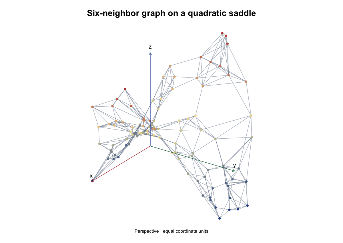
The figure uses the exact seed and sample above. Edges carry Euclidean chord lengths, not surface geodesic lengths. Color represents height, from blue (low) through cream to red (high). Its generation recipe also defines the labeled perspective view. The full geometry gallery compares forms, sampling densities, coordinate frames and dimensions.
Geometry-only samples contain coordinates, geometric metadata and reproducible random-state information. Statistical truth, responses, named recipe registries and dataset identities remain in geosmooth. The forthcoming geosmooth release imports these geometry helpers from dgraphs. The development Geometry Lab app is documented in dev/apps/embedding-explorer/README.md; it is not installed with the R package.
Graph Reconstruction Explorer
Open saved graph reconstruction benchmarks with dgraphs::explore.graphs(). The optional app dependencies are shiny, bslib, plotly, and digest. Use explore.graphs(project = run_directory) to open an existing benchmark, or remember it with register.graph.project(run_directory, name = "My study"). The no-argument launcher presents your saved projects. Scientific data stay outside the package; opening them does not rerun analysis. grip is needed only when you explicitly generate a missing weighted layout.
Start with the bundled twelve-point circle comparison:
install.packages(c("shiny", "bslib", "plotly", "digest"))
demo <- system.file("extdata", "graph-explorer-demo", package = "dgraphs")
benchmark <- read.graph.benchmark(demo)
explore.graphs(demo)
Compare k = 2 and k = 4: extra chords increase error relative to exact circle arcs. Both graph layouts and metric tables are saved, so this demonstration needs no fitting or project registration. The default display preserves coordinate proportions, with labeled x/y/z axes. See ?explore.graphs for project paths and cache controls.