Density-sensitive paths with Fermat distances • dgraphs

The estimator and its graph restriction

The sample Fermat distance between observed points minimizes the sum of powered Euclidean step lengths over all sequences of observed points:

$D_p(i,j)=\min_{\pi:i\leadsto j}\sum_{(a,b)\in\pi}\|x_a-x_b\|^p.$

fermat.distances(points = X, p = 2) computes this complete-graph reference. It does not first remove long edges. For p > 1, several short steps can cost less than a single long step. This favors densely sampled routes without explicitly fitting a density estimate. For p = 1, the complete-graph answer is Euclidean distance, not distance around a circle.

The default result is the unrooted sum. rooted = TRUE takes its 1/p power: this changes reported distances but not minimizing paths. Neither option applies sample-size normalization or estimates a limiting constant.

X <- matrix(c(0, 1, 2), ncol = 1)
fermat.distances(points = X, p = 2)
#>      [,1] [,2] [,3]
#> [1,]    0    1    2
#> [2,]    1    0    1
#> [3,]    2    1    0

The distance from 0 to 2 is 2: the two unit steps cost less than the direct step, which costs 4.

Two explicit restrictions are also available:

fermat.distances(points = X, graph.type = "sknn", k = 1, p = 2)
#>      [,1] [,2] [,3]
#> [1,]    0    1    2
#> [2,]    1    0    1
#> [3,]    2    1    0
graph <- create.sknn.graph(X, k = 1, neighbor.method = "exact",
                          prune.edges = FALSE, connect.components = FALSE)
fermat.distances(graph, p = 2)
#>      [,1] [,2] [,3]
#> [1,]    0    1    2
#> [2,]    1    0    1
#> [3,]    2    1    0

Coordinate kNN construction uses union symmetrization: either endpoint may select an edge. Supplied graphs use their stored lengths as base lengths before powering. With the same retained weights, restricting edges cannot decrease the distance. Missing routes return Inf; no connectivity repair is implicit. Use vertices = c(i, j) for a selected submatrix; paths still use other vertices.

Noisy circles with different sampling densities

We generate 100 observations around a unit circle with radial Gaussian noise of standard deviation 0.04. One example has uniform angular sampling; the other places half the observations near angle zero. Both retain a uniform angular component. These are fixed illustrations, not a simulation study or a proof of geometric recovery. Radial noise changes the sampled geometry from an exact circle; circle arc length is therefore not a universal truth target.

set.seed(4101)
n <- 100
angles <- list(
  Uniform = sort(runif(n, 0, 2*pi)),
  Concentrated = sort(c(runif(n/2, 0, 2*pi),
                        rnorm(n/2, 0, 0.4) %% (2*pi)))
)
radial.noise <- rnorm(n, 0, 0.04)
circles <- lapply(angles, function(theta) {
  cbind((1 + radial.noise)*cos(theta), (1 + radial.noise)*sin(theta))
})
powers <- c(1, 2, 3)
reference <- lapply(circles, function(X) {
  lapply(powers, function(p) fermat.distances(points = X, p = p))
})

To visualize the minimizing routes, the next chunk uses igraph on the same complete graph and powered Euclidean weights. It checks each plotted path’s cost against fermat.distances(). Black points mark the selected endpoints; red segments show a shortest path. Tied minimizers may have different shapes. Notice how the preferred route changes with the power and sampling pattern; a dense route need not be the shortest circular arc.

old <- par(mfrow = c(2, 3), mar = c(3, 3, 2, 0.5))
for (s in seq_along(circles)) {
  X <- circles[[s]]
  ends <- c(which.min(rowSums(sweep(X, 2, c(1,0), "-")^2)),
            which.min(rowSums(sweep(X, 2, c(-1,0), "-")^2)))
  g <- igraph::make_full_graph(n, directed = FALSE)
  e <- igraph::as_edgelist(g, names = FALSE)
  eu <- as.matrix(dist(X))
  for (j in seq_along(powers)) {
    p <- powers[j]
    weights <- eu[e]^p
    path <- as.integer(igraph::shortest_paths(g, from = ends[1], to = ends[2],
                                             weights = weights)$vpath[[1]])
    cost <- sum(eu[cbind(head(path, -1), tail(path, -1))]^p)
    stopifnot(isTRUE(all.equal(cost, reference[[s]][[j]][ends[1],ends[2]])))
    plot(X, asp = 1, pch = 16, cex = 0.5, col = "gray60",
         xlab = "x", ylab = "y", main = paste(names(circles)[s], "p =", p))
    lines(X[path, , drop = FALSE], col = "firebrick", lwd = 2)
    points(X[ends, ], pch = 16, cex = 1.1)
  }
}

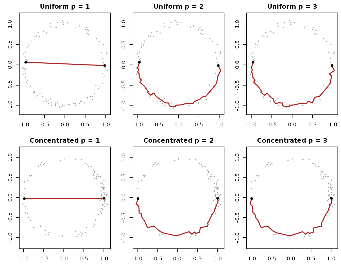
Six circle panels compare complete-graph paths for three powers and two angular sampling distributions. Endpoints are black, observations gray, and minimizing paths red.

Complete-graph shortest paths at powers 1, 2 and 3. Rows show uniform and concentrated angular sampling; axes are the observed Cartesian coordinates.

par(old)

Does a sparse graph give the same distances?

For each circle and power, compare symmetric kNN restrictions at k = 4, 8, 16 against all unordered pairs of the complete reference. The table reports unreachable pairs separately. Relative error is measured only for finite restricted distances; it does not hide disconnections. Numerical agreement uses tolerance 1e-10 * max(1, reference distance).

rows <- list()
for (s in seq_along(circles)) for (j in seq_along(powers)) {
  full <- reference[[s]][[j]]
  use <- upper.tri(full)
  for (k in c(4, 8, 16)) {
    restricted <- fermat.distances(points = circles[[s]], p = powers[j],
                                   graph.type = "sknn", k = k)
    finite <- use & is.finite(restricted)
    stopifnot(all(restricted[use] >= full[use] - 1e-10))
    agree <- is.finite(restricted[use]) &
      abs(restricted[use] - full[use]) <= 1e-10*pmax(1, full[use])
    rows[[length(rows)+1L]] <- data.frame(
      Sampling = names(circles)[s], p = powers[j], k = k,
      Unreachable = sum(use & !is.finite(restricted)),
      Agreement_percent = 100*mean(agree),
      Max_relative_error = if (any(finite))
        max(abs(restricted[finite] - full[finite])/full[finite]) else NA_real_
    )
  }
}
knitr::kable(do.call(rbind, rows), digits = 4)

Sampling	p	k	Agreement_percent	Max_relative_error
Uniform	1	4	4.6869	39.4228
Uniform	1	8	8.9899	0.6082
Uniform	1	16	17.5152	0.5792
Uniform	2	4	51.4343	32.9562
Uniform	2	8	100.0000	0.0000
Uniform	2	16	100.0000	0.0000
Uniform	3	4	66.9697	30.1992
Uniform	3	8	100.0000	0.0000
Uniform	3	16	100.0000	0.0000
Concentrated	1	4	4.9495	20.1804
Concentrated	1	8	9.4343	0.5957
Concentrated	1	16	19.2525	0.5321
Concentrated	2	4	78.0808	11.8217
Concentrated	2	8	100.0000	0.0000
Concentrated	2	16	100.0000	0.0000
Concentrated	3	4	86.1414	9.5385
Concentrated	3	8	100.0000	0.0000
Concentrated	3	16	100.0000	0.0000

Agreement in this table establishes equivalence only for these finite samples, powers and neighborhood sizes. In particular, the p = 1 rows demonstrate that circle-following kNN distances can differ from the Euclidean reference. Increasing k to n - 1 always restores the complete graph, at quadratic storage cost. Merely observing no change between two smaller k values does not certify equivalence to the reference.

Two noisy arms with diffuse background points

The circle illustrates a change in distance. Two arms ask a different question: when does density make a path follow populated structures instead of crossing between them? We use two perpendicular segments of length one, with 80 samples per arm. Radial coordinates are uniform on [0,1]; transverse displacements are independent absolute Gaussian draws with scale 0.005. There is no supplied junction vertex. Background points are uniform in the unit square, not placed on translated rows and not assigned to an arm.

We compare 20 and 120 background points. The smaller set is contained in the larger, and all arm observations and endpoint identities stay fixed. The seed, width, background levels and endpoint-selection rule were fixed before inspecting paths. This is the first seed of a separate 12-seed exploratory comparison at three widths (0.005, 0.02, 0.05) and three background counts (20, 60, 120), not a seed selected for its appearance.

The installed teaching helper below contains the generator, deterministic pair selection, geometric scoring and plotting code. It is a script, not an exported package API. Its source can be inspected at the path returned by system.file().

source(system.file("examples", "fermat-two-arms.R", package = "dgraphs"))
arm.examples <- lapply(c(20L, 120L), function(count) {
  fermat.two.arms(seed = 6101L, width = 0.005, background = count)
})
arm.routes <- lapply(arm.examples, function(sample) {
  lapply(1:3, function(p) fermat.arm.paths(sample, p))
})

We evaluate ten arm-endpoint pairs away from the junction and up to twelve background pairs from the first twenty background points. Background endpoints must lie more than 0.08 from either axis and have different nearest axes. Pairs are ranked by closeness to targets (0.65,0.18) and (0.18,0.65), before any path calculation. Only the first pair of each kind is plotted; the distance checks below use every evaluated pair. The background endpoints’ distances to the nearest arm are shown here, in units where an arm has length one.

sample <- arm.examples[[1]]
ends <- sample$background.pairs[1, ]
knitr::kable(data.frame(Endpoint = c("Start", "End"),
                       x = sample$X[ends,1], y = sample$X[ends,2],
                       Distance_to_arm = apply(sample$X[ends,,drop=FALSE],1,min)),
             digits = 3)

Endpoint	x	y	Distance_to_arm
Start	0.633	0.354	0.354
End	0.081	0.461	0.081

For each polygonal path gamma, the junction indicator is $J=\mathbf{1}\{\min_{z\in\gamma}\|z\|\leq0.1\}$ . This checks the whole path, not only its vertices. Let $T=([0,1]\times[0,0.05])\cup([0,0.05]\times[0,1])$ . Arm coverage is $A=\operatorname{length}(\gamma\cap T)/\operatorname{length}(\gamma)$ , using Euclidean segment length, not the powered cost. The score is between zero and one. Higher coverage means more travel near the arms; neither score is a universal measure of correctness. Segment intersections with the two rectangles are computed exactly up to floating-point arithmetic.

Blue points are arm observations, gray crosses are diffuse background, black circles are endpoints, and red lines are minimizing paths. Shading marks T; the dashed quarter-circle marks the junction disk. All panels use observed coordinates and complete-graph powered Euclidean costs.

old <- par(mfrow = c(2,3), mar = c(3,3,2,0.5))
for (s in 1:2) for (p in 1:3) {
  fermat.plot.arm.path(arm.examples[[s]], arm.routes[[s]][[p]]$paths[[1]],
                      paste(arm.examples[[s]]$background, "background; p =", p))
}

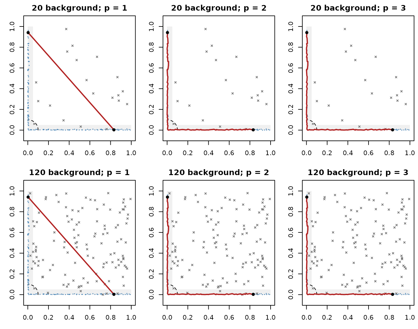
Six two-arm panels show complete-graph paths between fixed arm endpoints, comparing two nested background levels and three powers.

Paths between arm observations. Rows contain 20 and 120 background points; columns show powers 1, 2 and 3. The arm sample and endpoints are fixed across panels.

par(old)

old <- par(mfrow = c(2,3), mar = c(3,3,2,0.5))
for (s in 1:2) for (p in 1:3) {
  index <- nrow(arm.examples[[s]]$arm.pairs) + 1L
  fermat.plot.arm.path(arm.examples[[s]], arm.routes[[s]][[p]]$paths[[index]],
                      paste(arm.examples[[s]]$background, "background; p =", p))
}

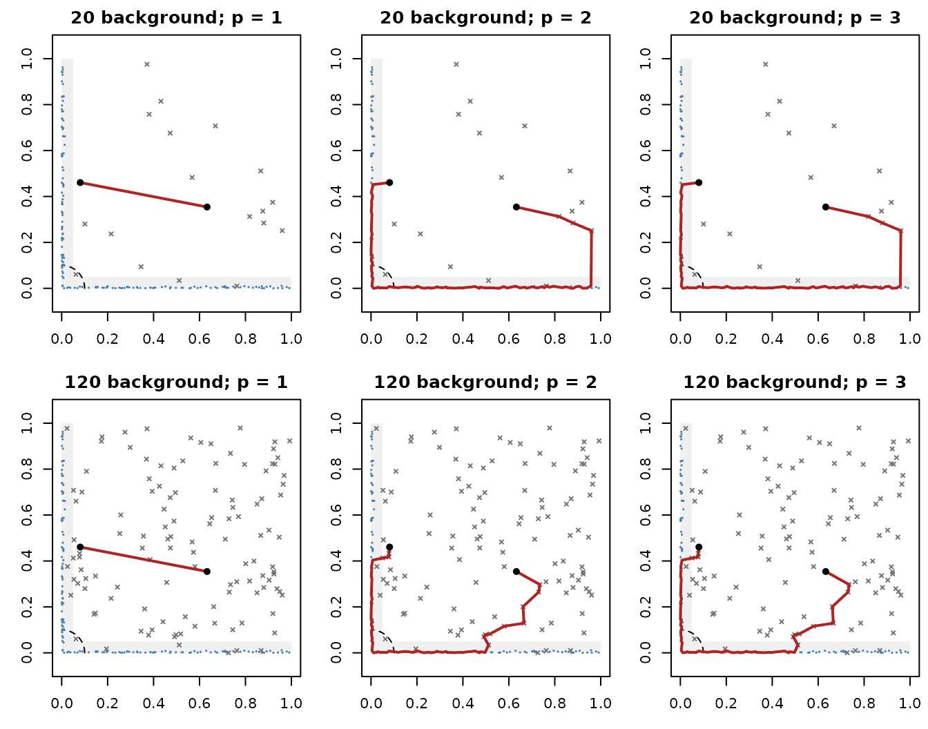
Six panels show paths between two fixed diffuse background observations near different arms, with 20 or 120 background points and powers 1, 2 and 3.

Paths between background observations near different arms, with the same samples and visual encodings. Endpoints are fixed and are not assigned generating-arm labels.

par(old)

The next table describes the twelve displayed paths. Junction entry is a yes/no indicator, and arm coverage is a percentage of the entire path’s Euclidean length, including its endpoint attachments. Thus background paths can follow the arms between attachments without reaching 100% coverage.

shown <- do.call(rbind, lapply(1:2, function(s) do.call(rbind,lapply(1:3,function(p) {
  scores <- arm.routes[[s]][[p]]$scores[c(1,11),]
  data.frame(Background=arm.examples[[s]]$background, Power=p,
             Endpoints=scores$type, Junction=ifelse(scores$junction==1,"Yes","No"),
             Arm_coverage_percent=100*scores$arm.fraction)
}))))
knitr::kable(shown, digits=1)

Background	Power	Endpoints	Junction	Arm_coverage_percent
20	1	Arm endpoints	No	10.7
20	1	Background endpoints	No	0.0
20	2	Arm endpoints	Yes	100.0
20	2	Background endpoints	Yes	72.7
20	3	Arm endpoints	Yes	100.0
20	3	Background endpoints	Yes	72.7
120	1	Arm endpoints	No	10.7
120	1	Background endpoints	No	0.0
120	2	Arm endpoints	Yes	100.0
120	2	Background endpoints	Yes	63.0
120	3	Arm endpoints	Yes	100.0
120	3	Background endpoints	Yes	63.0

These plots separate density preference from obligatory attachment. Adding background creates potential travel routes between the arms. Such a route is not automatically an estimator error: the background is part of the sampled support. In particular, a finite density-sensitive distance need not take nearby background points to an arm and back.

We also check the same endpoint pairs with symmetric kNN restrictions. Agreement means absolute error at most 1e-10 * max(1, complete distance). The table gives percent agreement over the selected pairs, separately for k=8 and k=16; nonfinite distances count as disagreements. The unreachable count sums across both restrictions. Each igraph path cost is independently checked against the package’s complete-graph calculation.

arm.agreement <- list()
for (s in 1:2) for (p in 1:3) {
  result <- arm.routes[[s]][[p]]
  vertices <- sort(unique(as.vector(result$pairs)))
  index <- cbind(match(result$pairs[,1],vertices),match(result$pairs[,2],vertices))
  full <- fermat.distances(points=arm.examples[[s]]$X,p=p,vertices=vertices)[index]
  stopifnot(max(abs(full-result$scores$cost)) < 1e-10)
  restricted <- lapply(c(8,16),function(k) {
    fermat.distances(points=arm.examples[[s]]$X,p=p,vertices=vertices,
                     graph.type="sknn",k=k)[index]
  })
  agree <- vapply(restricted,function(d) {
    stopifnot(all(d >= full-1e-10))
    100*mean(is.finite(d) & abs(d-full)<=1e-10*pmax(1,full))
  },0)
  arm.agreement[[length(arm.agreement)+1L]] <- data.frame(
    Background=arm.examples[[s]]$background, Power=p, Pairs=length(full),
    Agreement_k8_percent=agree[1], Agreement_k16_percent=agree[2],
    Unreachable=sum(!is.finite(unlist(restricted))))
}
knitr::kable(do.call(rbind,arm.agreement),digits=1)

Background	Power	Pairs	Agreement_k8_percent	Agreement_k16_percent
20	1	22	4.5	4.5
20	2	22	100.0	100.0
20	3	22	100.0	100.0
120	1	22	0.0	0.0
120	2	22	100.0	100.0
120	3	22	100.0	100.0

Any equivalence shown here applies to these selected pairs only. The circle comparison above checks all pairs. A connected graph or an attractive path plot does not certify that a restriction preserves Fermat distances.

How much does the first seed conceal?

The displayed pair follows the arms at powers 2 and 3 under both background levels. To show its limits, the next calculation repeats power 2 over the predeclared twelve seeds, at the narrowest and broadest arm widths and both background levels. Each seed contributes its mean over ten arm pairs or twelve background pairs; endpoint pairs are not treated as independent replicates. The table gives means and 95% percentile bootstrap intervals from 2,000 seed resamples. Width is the pre-folding Gaussian scale; both path scores are percentages. Degenerate intervals do not imply certainty for future samples.

seed.scores <- list()
for (seed in 6101:6112) for (width in c(0.005,0.05)) for (count in c(20L,120L)) {
  sample <- fermat.two.arms(seed, width, count)
  scores <- fermat.arm.paths(sample, p=2)$scores
  means <- aggregate(scores[c("junction","arm.fraction")],list(Endpoints=scores$type),mean)
  means$Seed <- seed; means$Width <- width; means$Background <- count
  seed.scores[[length(seed.scores)+1L]] <- means
}
seed.scores <- do.call(rbind,seed.scores)
set.seed(8201)
mean.interval <- function(x) {
  boot <- replicate(2000,mean(sample(x,replace=TRUE)))
  sprintf("%.1f (%.1f–%.1f)",100*mean(x),
          100*quantile(boot,.025),100*quantile(boot,.975))
}
seed.summary <- do.call(rbind,lapply(split(seed.scores,
  interaction(seed.scores[c("Width","Background","Endpoints")],drop=TRUE)),function(d) {
    data.frame(d[1,c("Width","Background","Endpoints")],
               Junction_percent=mean.interval(d$junction),
               Arm_coverage_percent=mean.interval(d$arm.fraction))
}))
rownames(seed.summary) <- NULL
knitr::kable(seed.summary)

Width	Background	Endpoints	Junction_percent	Arm_coverage_percent
0.005	20	Arm endpoints	100.0 (100.0–100.0)	100.0 (100.0–100.0)
0.050	20	Arm endpoints	50.0 (25.0–75.0)	78.6 (73.5–82.9)
0.005	120	Arm endpoints	100.0 (100.0–100.0)	100.0 (100.0–100.0)
0.050	120	Arm endpoints	41.7 (16.7–66.7)	75.1 (69.2–80.6)
0.005	20	Background endpoints	45.1 (30.6–61.1)	35.6 (24.0–47.6)
0.050	20	Background endpoints	22.9 (7.6–41.0)	30.2 (21.2–38.8)
0.005	120	Background endpoints	22.2 (11.8–33.3)	18.1 (10.0–27.1)
0.050	120	Background endpoints	6.9 (0.0–15.3)	11.2 (5.6–17.7)

For narrow arms, every tested arm-to-arm path at power 2 visits the junction, whereas background-to-background visits average only 45.1% with 20 background points and 22.2% with 120. Wider arms weaken junction routing further. The fixed width-0.05 coverage rectangles contain less of the broad clouds, so falling coverage alone is not evidence of additional shortcuts.

The first-seed distance-agreement table likewise establishes only what was checked in that realization. It is not a guarantee for subsequent datasets.

Complete-graph distances without storing the graph

backend = "implicit" retains the complete-graph estimator but computes edge costs during dense Dijkstra searches. It avoids quadratic adjacency storage. Selecting source vertices (pivots) also avoids an all-pairs output matrix; every observation can still occur inside a minimizing path.

X <- circles[[1]]
pivots <- c(1L, 14L, 27L, 40L, 53L, 66L, 79L, 92L)
pivot.distances <- fermat.distances(points = X, p = 2,
    backend = "implicit", sources = pivots)
stopifnot(isTRUE(all.equal(pivot.distances,
                          reference[[1]][[2]][pivots, , drop = FALSE])))
dim(pivot.distances)
#> [1]   8 100
# Rectangular queries preserve the supplied row and column order.
fermat.distances(points = X, backend = "implicit", sources = pivots[1:2],
                targets = c(25L, 50L, 75L))
#>           [,1]      [,2]      [,3]
#> [1,] 0.3585997 0.3261286 0.1878795
#> [2,] 0.1962370 0.3457390 0.3502421

With h sources, n observations and d coordinates, worst-case work is O(h n² d), plus an O(n² d) numeric-range check. Memory is O(n d + h n) for source-to-all queries. Requesting all sources still produces an n-by-n matrix. max.workspace.bytes checks an estimate of input, output and native scratch storage; it is not a cap on total R process memory. This backend trades repeated edge evaluation for less storage; it does not promise subquadratic search time or approximate the missing distances.

Sparse metric MDS with consistent Fermat targets

The teaching helper below constructs local symmetric kNN pairs and pivot interactions. Both receive complete-graph Fermat distances. In particular, a local pair’s target can be smaller than its powered direct-edge length. The helper uses nearest-pivot regions and half-distance region counts for asymmetric long-range weights, with unit endpoint multiplicities for local pairs, following the weighting construction used by grip’s sparse mode. Pivots here are fixed observation indices, not graph-distance random samples.

source(system.file("examples", "fermat-sparse-mds.R", package = "dgraphs"))
constraints <- fermat.mds.constraints(X, pivots, k = 4, p = 2)
stopifnot(max(abs(constraints$targets -
                 reference[[1]][[2]][constraints$pairs])) < 1e-10)
c(retained = nrow(constraints$pairs), all.pairs = choose(nrow(X), 2))
#>  retained all.pairs 
#>       960      4950

With a grip version supporting explicit constraints, fit these targets as follows. Sparse fitting approximates the embedding objective; the supplied Fermat targets themselves are exact sample distances, up to arithmetic.

fit <- grip::metric.mds(n = nrow(X), approximation = "sparse",
                       constraints = constraints, seed = 1, max.iter = 100)
plot(fit$coords, asp = 1, pch = 16)

The helper is a readable teaching implementation, not a fast neighbor-search API. Its local targets require additional source searches with early stopping; worst-case preparation can still be cubic in n. It never allocates an all-pairs distance matrix. Inverse-squared MDS weights require positive targets, so consolidate coincident observations first; the Fermat distance function itself continues to support them. Evaluate embedding fidelity on independent pairs, not only the constraints used for fitting.

What the theory does and does not establish

Groisman, Jonckheere and Sapienza define the unrooted complete-graph estimator and establish a normalized continuum limit under their sampling assumptions. They also define directed nearest-neighbor restrictions and prove a high-probability equality with the unrestricted estimator when k exceeds a bound of the form c1 * log(n / epsilon) + c2, under the stated hypotheses (Definitions 2.1 and 2.11, Proposition 2.12). This does not select a certified finite-sample k for these noisy examples.

Union-symmetric kNN contains the directed edges, so equality for the directed restriction implies equality for the union restriction by inclusion of paths. Arbitrary pruning, mutual-neighbor intersections and other supplied graphs need separate justification. A rooted output is a transformation of the unrooted estimator and must be interpreted with its corresponding scaling.

This example tests graph restriction directly rather than assuming it is harmless. Further assessment should use multiple sample sizes and seeds, and should distinguish recovering ordinary geometry from deliberately changing distances through sampling density. Neither a visually appealing path nor a connected graph establishes the continuum theorem’s assumptions.

The explicit complete-graph backend and all-pairs output require quadratic storage. The implicit backend avoids adjacency storage. Both fermat.distances() coordinate graph constructions still evaluate all Euclidean pairs; kNN restriction reduces the stored graph, not that neighbor-search work. Start with small reference examples. Positive lengths that overflow or underflow to zero after powering are rejected; rescale the coordinates if necessary.

Exact nearest neighbors without all-pairs distances

When the desired output is a neighborhood graph, fermat.knn() finds each observation’s nearest neighbors in the complete-graph Fermat distance. It caches exact Euclidean neighbor lists and uses truncated Dijkstra searches. This is a separate operation from asking fermat.distances(graph.type = "sknn") for a matrix of arbitrary pairwise distances.

McKenzie and Damelin’s Lemma 5.6 justifies pruning for these local queries: the neighbor distances are those of the complete graph. It does not assert that the resulting sparse graph preserves every pairwise distance. Our k counts other observations, while the paper includes the source in its count.

set.seed(193)
neighbor.points <- matrix(runif(120), 60, 2)
neighbors <- fermat.knn(neighbor.points, k = 6, p = 2)
neighbor.graph <- create.fermat.sknn.graph(neighbor.points, k = 6, p = 2)
reference <- fermat.distances(points = neighbor.points, p = 2)
selected <- cbind(rep(seq_len(nrow(neighbor.points)), 6),
                  as.vector(neighbors$index))
stopifnot(max(abs(as.vector(neighbors$distance) - reference[selected])) < 1e-10)

The graph takes the union of directed selections: an edge remains if either endpoint selected the other. Its stored lengths are the computed Fermat distances. Do not power those lengths again when calculating graph geodesics. Union symmetrization can give a vertex more than k neighbors; connectivity is not forced. Equal-distance ties at the cutoff may produce different valid neighbor selections. Coincident observations remain separate vertices.

Candidate storage grows as n * k. Once candidates are available, binary-heap path searches cost approximately n * k^2 * log(k + 1). Exact Euclidean search can still be expensive in high dimensions. The search offers exact k-d tree and brute-force options; neither uses approximate neighbors. Pivot-to-all queries still use the separate implicit backend.

References

Groisman, P., Jonckheere, M. and Sapienza, F. (2022). Nonhomogeneous Euclidean first-passage percolation and distance learning. Bernoulli 28(1), 255–276. Published paper and preprint with definitions and propositions.

For ordinary graph distances and graph construction, see Constructing and Diagnosing Data-Derived Graphs.

McKenzie, D. and Damelin, S. (2019). Power Weighted Shortest Paths for Clustering Euclidean Data. Preprint, section 5.