Synthetic geometry and point sampling

A synthetic point cloud begins with two choices: a geometry describes where points can lie, and a sampling specification describes how to choose them. Constructing either specification performs no random draws. sample.synthetic.geometry() realizes the points under an explicit seed or random-state plan. This separation lets you change sampling density while keeping the underlying geometry fixed.

dgraphs owns reusable geometry, point sampling, embeddings and graph tools. Statistical truth, response generation, statistical recipes, dataset registry identities and model fitting belong to geosmooth. That package can combine these geometric components with truth and response specifications; it is not needed to run any example here. The development Geometry Lab application is not an installed package function. Its two exported arithmetic/sampling helpers are documented below because they are part of the public API.

A curve: angles, coordinates and a graph

A circle has one latent coordinate, its angle, and two ambient coordinates. The interval-grid sampler is deterministic; excluding its lower endpoint avoids duplicating the point at angles zero and two pi.

library(dgraphs)
circle <- synthetic.circle(radius = 1, ambient.dim = 2)
grid <- synthetic.sampling.grid.interval(
  0, 2 * pi, endpoints = "exclude.lower"
)
cloud <- sample.synthetic.geometry(circle, grid, n = 32, seed = 2026)
c(latent.columns = ncol(cloud$latent),
  ambient.columns = ncol(cloud$predictors))
#>  latent.columns ambient.columns 
#>               1               2
stopifnot(isTRUE(all.equal(
  embed.synthetic.geometry(circle, cloud$latent), cloud$predictors
)))
graph <- create.sknn.graph(cloud$predictors, k = 2,
                           connect.components = TRUE)
edges <- convert.adjacency.to.edge.matrix(graph.adjacency(graph))$edge.matrix

X <- cloud$predictors
plot(X, asp = 1, pch = 19, col = "#245A81", xlab = "x", ylab = "y")
segments(X[edges[, 1], 1], X[edges[, 1], 2],
         X[edges[, 2], 1], X[edges[, 2], 2], col = "grey50")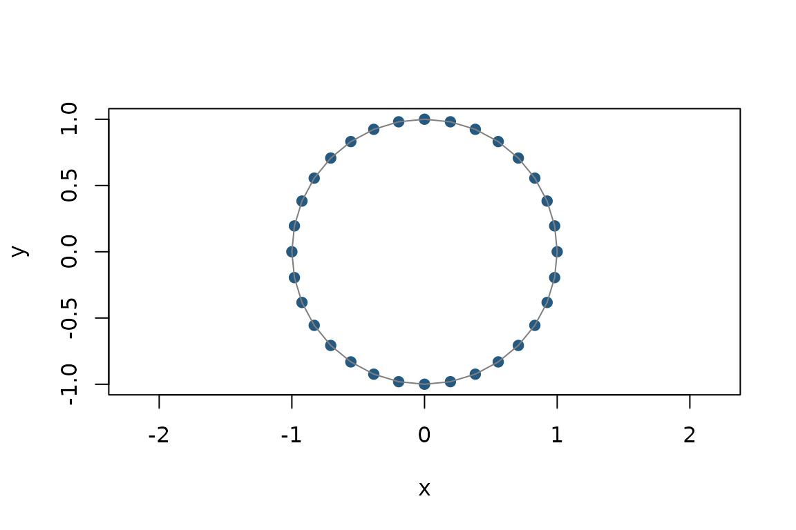

Circle sample with edges between nearby observations. Each coordinate row is a graph vertex.

The graph uses Euclidean chord lengths. Its shortest-path distance sums those lengths along graph edges. The continuous circle distance instead uses the shorter circular arc. Compare one quarter-turn:

D <- graph.geodesic.distances(graph)
angle <- abs(cloud$latent[1, 1] - cloud$latent[9, 1])
c(chord = sqrt(sum((X[1, ] - X[9, ])^2)),
  graph.path = D[1, 9],
  circle.arc = min(angle, 2 * pi - angle))
#>      chord graph.path circle.arc 
#>   1.414214   1.568274   1.570796

The graph path approximates the arc as sampling becomes dense enough and neighborhoods remain local. Sparse or overly large neighborhoods can produce gaps or shortcuts. Connectivity repair can bridge gaps, but does not certify that a bridge respects the intended continuous geometry.

A quadratic surface: parameter sampling and embedding

A quadratic geometry has intrinsic.dim latent coordinates and ambient.dim embedded coordinates. Each symmetric matrix in forms defines a height z' Q z, without a factor of one half. No forms gives a flat geometry. Multiple forms give multiple height coordinates, requiring room in the ambient dimension for the latent coordinates and all heights.

saddle <- synthetic.quadform(
  intrinsic.dim = 2, ambient.dim = 3, forms = list(diag(c(1, -1)))
)
sampling <- synthetic.sampling.uniform.disk(radius = 1)
validate.synthetic.sampling(sampling, saddle)
surface <- sample.synthetic.geometry(saddle, sampling, n = 48, seed = 17)
head(cbind(surface$latent, height = surface$predictors[, 3]), 3)
#>                                    height
#> [1,]  0.1779531177  0.1374088  0.01278613
#> [2,] -0.0001947751 -0.8769291 -0.76900463
#> [3,]  0.2274133632  0.5230924 -0.22190877
surface.graph <- create.sknn.graph(surface$predictors, k = 5,
                                   connect.components = TRUE)
length(unique(graph.connected.components(surface.graph)))
#> [1] 1

Uniform disk draws are uniform in the latent disk’s area, not in the curved surface’s area. synthetic.sampling.quadform.lab(domain = "disk", mode = "area") uses rejection sampling for surface area. That specialized sampler requires a canonical two-dimensional quadratic surface in three dimensions, zero offset, coefficients in [-20, 20], and its documented extent limits. Its other modes include uniform, grid, center and gap sampling. embed.quadform.surface() likewise preserves the versioned Geometry Lab arithmetic for a two-column input and three coefficients.

Chords, lifted segments and shortest paths

edge.lengths.synthetic.geometry() currently accepts quadforms only. It measures the curve obtained by lifting a straight latent segment onto the surface. That curve need not be the shortest continuous surface path. Graph constructors do not automatically replace their Euclidean chord weights with these lifted-segment lengths.

a <- matrix(c(-0.8, 0), nrow = 1)
b <- matrix(c(0.8, 0), nrow = 1)
A <- embed.synthetic.geometry(saddle, a)
B <- embed.synthetic.geometry(saddle, b)
c(ambient.chord = sqrt(sum((B - A)^2)),
  lifted.segment = edge.lengths.synthetic.geometry(saddle, a, b))
#>  ambient.chord lifted.segment 
#>       1.600000       2.133929
quadform.metric(saddle, a)
#>      [,1] [,2]
#> [1,] 3.56    0
#> [2,] 0.00    1

The induced metric describes local length in latent coordinates. quadform.gradient() returns an n by d matrix for one height, an n by r by d array for r heights, and an n by zero by d array for no heights. quadform.metric() returns a d by d matrix for one point and an n by d by d array for multiple points. These shape differences are intentional.

Random frames and single points

A random orthonormal frame changes the ambient orientation. The sampler returns its realized frame.matrix. Reuse that matrix when embedding another set of latent points; embed.synthetic.geometry() itself performs no random draws and requires the realized matrix for a random-frame geometry.

rotated <- synthetic.quadform(
  intrinsic.dim = 2, ambient.dim = 5,
  forms = list(diag(c(1, -1)), diag(c(0.5, 0.25))),
  frame = "random.orthonormal"
)
one <- sample.synthetic.geometry(
  rotated, synthetic.sampling.uniform.box(-1, 1), n = 1, seed = 91
)
dim(one$latent)
#> [1] 1 2
dim(one$predictors)
#> [1] 1 5
stopifnot(identical(dim(one$latent), c(1L, 2L)),
          identical(dim(one$predictors), c(1L, 5L)),
          isTRUE(all.equal(one$predictors,
            embed.synthetic.geometry(rotated, one$latent, one$frame.matrix))))

One-point box samples retain matrix dimensions, including embeddings with multiple heights. This does not imply that a nearest-neighbor graph constructor accepts a single observation: its own size and k constraints still apply.

Explore quadratic geometry in 3D

The galleries below use ivue to display coordinates generated by dgraphs. Choose an example, drag to rotate, and use the mouse wheel or trackpad to zoom. Reset view restores that example’s initial camera. Each view has labeled x, y and z axes, uses equal data-unit scales, and starts with z pointing upward. A displayed mesh is a piecewise-planar drawing aid, not a new graph or an exact continuous surface.

To rebuild interactive views, install ivue and its optional rgl backend. The ivue source is available from its package repository. The numerical examples execute independently of ivue. Builds without the optional visualization packages show labeled static perspective views instead; an HTML built with ivue contains its interactive views and needs only a WebGL-capable browser to read it, with no running R or Shiny session.

For a single view in your own R session, the sampled saddle above can be drawn with this short call. The galleries add meshes, selectors and captions around the same ivue plotting functions.

ivue::plot3D.cont(
  surface$predictors, values = surface$predictors[, 3],
  legend.title = "Height", aspect = "equal",
  layers = list(ivue::layer3D.axes(labels = c("x", "y", "z"))),
  camera = ivue::camera.zup(elevation = 25, turn = -125, zoom = 0.53)
)

Shape: flat, bowl, dome, cylinder, saddle and mixed terms

For two latent coordinates u, v, a symmetric form Q = matrix(c(a, b, b, c), 2) gives h(u, v) = a*u^2 + 2*b*u*v + c*v^2. The off-diagonal coefficient appears twice. Eigenvalue signs distinguish bowls, domes, saddles and cylinders; changing their magnitudes changes curvature. A flat geometry has no height form rather than a mandatory zero form.

This small regular grid is used only to draw surfaces. Two triangles per latent grid cell give known mesh connectivity without an additional triangulation package.

u <- seq(-1, 1, length.out = 15)
uv <- as.matrix(expand.grid(u = u, v = u))
cells <- expand.grid(i = seq_len(length(u) - 1L),
                     j = seq_len(length(u) - 1L))
a <- cells$i + (cells$j - 1L) * length(u)
faces <- rbind(cbind(a, a + 1L, a + length(u)),
               cbind(a + 1L, a + length(u) + 1L, a + length(u)))
forms <- list(
  Bowl = diag(c(1, 1)), Dome = diag(c(-1, -1)),
  Cylinder = diag(c(1, 0)), Saddle = diag(c(1, -1)),
  `Unequal curvature` = diag(c(0.25, 1.5)),
  `Mixed term` = matrix(c(0.4, 0.8, 0.8, -0.2), 2)
)
shape.views <- list()
flat <- synthetic.quadform(2, 2)
flat.X <- embed.synthetic.geometry(flat, uv)
shape.views$Flat <- quad.view(cbind(flat.X, 0),
  "No forms: two ambient coordinates, padded with z = 0 only for display.", faces)
for (name in names(forms)) {
    geometry <- synthetic.quadform(2, 3, forms = list(forms[[name]]))
    X <- embed.synthetic.geometry(geometry, uv)
    shape.views[[name]] <- quad.view(X, paste(name, "with x = u, y = v, z = the quadratic height."),
        faces)
}
shape.views <- shape.views[c("Saddle", setdiff(names(shape.views), "Saddle"))]
# The specialized arithmetic agrees numerically with the general embedding.
co <- c(0.4, 0.8, -0.2)
stopifnot(isTRUE(all.equal(shape.views[["Mixed term"]]$X,
                          embed.quadform.surface(uv, co), check.attributes = FALSE)))

Example: Saddle Flat Bowl Dome Cylinder Unequal curvature Mixed termReset view

Saddle with x = u, y = v, z = the quadratic height. Color: Displayed z; blue -1 to red 1.

Interactive 3D view of 225 observations.

embed.quadform.surface(uv, c(a, b, c)) is the specialized two-to-three coordinate lift. It has no frame or offset controls. The general synthetic.quadform() plus embed.synthetic.geometry() workflow supports the dimensions and placements illustrated below. Numerical agreement does not promise bitwise-identical arithmetic between these implementations.

Sampling: domain, density, gaps and ordering

The specialized sampler supports every combination of square/disk domain and five modes: uniform, area, grid, center and gap. All examples below use 180 points on the same saddle with an explicit seed. Use the selector to compare the ten combinations.

modes <- c("uniform", "area", "grid", "center", "gap")
sampling.views <- list()
for (domain in c("square", "disk")) for (mode in modes) {
    spec <- synthetic.sampling.quadform.lab(domain = domain, extent = 1, mode = mode, gap = 0.3)
    draw <- sample.synthetic.geometry(saddle, spec, n = 180, seed = 4101)
    stopifnot(nrow(draw$predictors) == 180L)
    if (mode == "gap")
        stopifnot(all(abs(draw$latent[, 1]) > 0.3))
    sampling.views[[paste(domain, mode, sep = " / ")]] <- quad.view(draw$predictors, paste("180 saddle points:",
        domain, "domain,", mode, "sampling."))
}
# General samplers support other domains, ordering and clustered designs.
general.samplers <- list(
  `Coordinate-wise box` = synthetic.sampling.uniform.box(
    lower = c(-1, -0.5), upper = c(1, 0.5), order = "ascending.first.coordinate"),
  Rectangle = synthetic.sampling.uniform.rectangle(c(-1, -0.5), c(1, 0.5)),
  `Uniform disk` = synthetic.sampling.uniform.disk(0.8),
  `Clustered points` = synthetic.sampling.clustered(6, 30, within.sd = 0.08)
)
for (name in names(general.samplers)) {
    draw <- sample.synthetic.geometry(saddle, general.samplers[[name]], n = 180, seed = 19)
    sampling.views[[name]] <- quad.view(draw$predictors, paste(name, "on the same quadratic saddle; no triangulation across gaps."))
}

Example: square / uniform square / area square / grid square / center square / gap disk / uniform disk / area disk / grid disk / center disk / gap Coordinate-wise box Rectangle Uniform disk Clustered pointsReset view

180 saddle points: square domain, uniform sampling. Color: Displayed z; blue -0.972 to red 0.902.

Interactive 3D view of 180 observations.

Control	Meaning and limitation
domain, extent	Square half-width or disk radius in latent coordinates; the specialized sampler requires extent in [0.1, 5].
uniform	Uniform latent-area sampling; surface area is larger in steeper regions.
area	Rejection sampling proportional to the induced surface-area element.
grid	A deterministic parameter grid, thinned to the exact requested count.
center	Rejection sampling concentrating points near the latent origin.
gap	Remove a strip with abs(u) <= gap * extent; gap lies in [0.01, 0.8].
algorithm	The specialized sampler accepts only "geometry.lab.v1"; its arithmetic and draw order are versioned.
General samplers	Boxes accept scalar or coordinate-wise bounds, rectangles draw two coordinates, disks use radial sampling, and clusters have fixed total size.
Ordering	Sorting a sample changes row/vertex identities, not its point set. Different sampler algorithms need not produce the same points for the same seed.

There is no mesh across the point samples: triangulating their convex hull would visually fill the deliberately empty strip. The specialized sampler requires exactly one quadratic height, a canonical 2D-to-3D geometry, zero offset and coefficients in [-20, 20]. For a rotated or translated version, sample canonically, then embed the stored latent coordinates using the desired frame and offset. The general samplers support those frames directly.

Placement: canonical, supplied and random frames, with offsets

A frame places the latent coordinates and heights in ambient space. Its columns must be orthonormal, so it rotates or reflects the canonical geometry without rescaling its distances. An offset translates the result. To rescale curvature, change the quadratic forms rather than supplying a nonorthonormal frame.

angle <- pi / 4
rotation <- matrix(c(1, 0, 0, 0, cos(angle), sin(angle),
                      0, -sin(angle), cos(angle)), 3)
placed <- synthetic.quadform(2, 3, list(diag(c(1, -1))),
  frame = "supplied", frame.matrix = rotation, offset = c(0.6, -0.3, 0.4))
placed.X <- embed.synthetic.geometry(placed, uv)
stopifnot(isTRUE(all.equal(as.matrix(dist(placed.X)),
                          as.matrix(dist(shape.views$Saddle$X)), tolerance = 1e-12)))
frame.views <- list(
  Canonical = shape.views$Saddle,
  `Supplied frame and translation` = quad.view(placed.X,
    "The same saddle rotated 45 degrees about x, then translated by (0.6, -0.3, 0.4). Axes remain ambient x/y/z.", faces)
)
for (algorithm in c("base.qr.gaussian.v1", "legacy.base.qr.gaussian.v1")) {
    geometry <- synthetic.quadform(2, 3, list(diag(c(1, -1))), frame = "random.orthonormal",
        frame.algorithm = algorithm)
    realization <- sample.synthetic.geometry(geometry, synthetic.sampling.uniform.box(-1, 1),
        n = 1, seed = 91)
    X <- embed.synthetic.geometry(geometry, uv, realization$frame.matrix)
    frame.views[[algorithm]] <- quad.view(X, paste("Random orthonormal orientation from seed 91 using",
        algorithm, "; frame.matrix is reused for every grid point."), faces)
}

Example: Canonical Supplied frame and translation base.qr.gaussian.v1 legacy.base.qr.gaussian.v1Reset view

Saddle with x = u, y = v, z = the quadratic height. Color: Displayed z; blue -1 to red 1.

Interactive 3D view of 225 observations.

The random frame is realized during sampling, not when the geometry is specified. Both supported frame algorithms are shown; the legacy spelling preserves historical draw contracts and is not an additional class of geometry. The canonical frame requires ambient.dim == intrinsic.dim + length(forms). Larger ambient dimensions require a supplied or random frame with shape ambient.dim by intrinsic.dim + length(forms).

Dimensions: a curve, multiple heights, a 3D latent domain and one point

A quadform need not be a surface in three dimensions. The next examples show the roles of both dimension arguments. Every view states whether it shows all coordinates, a projection or a slice. A 3D display cannot preserve all information about a geometry in four or more dimensions.

# One latent coordinate and two heights: all three ambient coordinates visible.
curve <- synthetic.quadform(1, 3, list(matrix(1), matrix(-0.4)))
curve.data <- sample.synthetic.geometry(curve,
  synthetic.sampling.grid.interval(-1, 1, endpoints = "include.both"),
  n = 61, seed = 2)
curve.edges <- cbind(1:60, 2:61)
dimension.views <- list(`Quadratic curve` = quad.view(curve.data$predictors,
  "One latent coordinate t, displayed as (t, t^2, -0.4 t^2). Both height coordinates are functions of t^2, so this curve lies in a plane.", edges = curve.edges))

# Two latent coordinates and two independent quadratic heights in four dimensions.
multi <- synthetic.quadform(2, 4,
  list(diag(c(1, -1)), matrix(c(0, 0.5, 0.5, 0), 2)))
X4 <- embed.synthetic.geometry(multi, uv)
stopifnot(identical(dim(quadform.gradient(multi, uv)), c(225L, 2L, 2L)))
dimension.views[["First of two heights"]] <- quad.view(X4[, c(1, 2, 3)],
  "Projection (u, v, h1) from four ambient coordinates; h2 = u*v is omitted.", faces,
  labels = c("x = u", "y = v", "z = h1"))
dimension.views[["Second of two heights"]] <- quad.view(X4[, c(1, 2, 4)],
  "Projection (u, v, h2) of the same rows; h1 = u^2-v^2 is omitted.", faces,
  labels = c("x = u", "y = v", "z = h2"))

# More ambient coordinates: an isometric supplied frame in five dimensions.
frame5 <- qr.Q(qr(rbind(diag(4), c(1, 1, 0, 0))))
wide <- synthetic.quadform(2, 5, multi$parameters$forms,
  frame = "supplied", frame.matrix = frame5, offset = c(0, 0, 0, 0, 0.5))
X5 <- embed.synthetic.geometry(wide, uv)
stopifnot(isTRUE(all.equal(as.matrix(dist(X4)), as.matrix(dist(X5)), tolerance = 1e-12)))
dimension.views[["Five-dimensional embedding"]] <- quad.view(X5[, c(1, 3, 5)],
  "Projection of ambient coordinates 1, 3 and 5. The full five-dimensional embedding preserves distances; this projection generally does not.", faces,
  labels = c("x = X1", "y = X3", "z = X5"))

# Three latent coordinates, one height: display two slices of a 4D geometry.
volume <- synthetic.quadform(3, 4,
  list(matrix(c(1, 0, 0.5, 0, -1, 0, 0.5, 0, 0.5), 3)))
volume.data <- sample.synthetic.geometry(volume,
  synthetic.sampling.uniform.box(-1, 1), n = 40, seed = 8)
stopifnot(identical(dim(volume.data$predictors), c(40L, 4L)))
for (w in c(-0.5, 0.5)) {
    slice <- embed.synthetic.geometry(volume, cbind(uv, w))
    dimension.views[[paste("Latent slice w =", w)]] <- quad.view(slice[, c(1, 2, 4)], paste("A two-dimensional slice at latent w =",
        w, "of a three-dimensional latent geometry; shown as (u, v, height)."), faces, labels = c("x = u",
        "y = v", "z = height"))
}
# The earlier one-point, two-height, random-frame sample is still a matrix.
dimension.views[["One point, five ambient coordinates"]] <- quad.view(
  one$predictors[, 1:3, drop = FALSE],
  "One row from a two-height geometry in five dimensions, projected to coordinates 1:3. A point alone does not identify the surrounding surface.")

Example: Quadratic curve First of two heights Second of two heights Five-dimensional embedding Latent slice w = -0.5 Latent slice w = 0.5 One point, five ambient coordinatesReset view

One latent coordinate t, displayed as (t, t^2, -0.4 t^2). Both height coordinates are functions of t^2, so this curve lies in a plane. Color: Displayed z; blue -0.4 to red 0.

Interactive 3D view of 61 observations.

The same quadform families also accept dimension-compatible interval samplers in one dimension, and box samplers in higher dimensions. Scalar box bounds, coordinate-wise bounds, a deterministic interval grid, disk/rectangle sampling and fixed-size clusters are illustrated above. For one-dimensional nonuniform designs, the existing truncated-normal and gapped-uniform specifications can be used without changing the geometry.

Differential geometry: gradient, metric and area element

For a two-dimensional surface with one height, the gradient describes its slope. The induced metric is I + gradient %*% t(gradient) at each point; its determinant gives the square of the local surface-area factor. Multiple heights contribute a sum of gradient outer products. Frames and offsets do not change this intrinsic metric.

gradient <- quadform.gradient(saddle, uv)
metric <- quadform.metric(saddle, uv)
slope <- sqrt(rowSums(gradient^2))
area.factor <- vapply(seq_len(nrow(uv)), function(i) sqrt(det(metric[i, , ])), numeric(1))
stopifnot(max(abs(area.factor - sqrt(1 + slope^2))) < 1e-12,
          identical(dim(quadform.gradient(flat, uv)), c(225L, 0L, 2L)),
          isTRUE(all.equal(quadform.metric(flat, matrix(c(0, 0), 1)), diag(2))))
differential.views <- list(
  `Gradient magnitude` = quad.view(shape.views$Saddle$X,
    "Slope increases away from the stationary point at the origin.", faces,
    values = slope, color.title = "Gradient magnitude"),
  `Surface-area factor` = quad.view(shape.views$Saddle$X,
    "This area factor is the density adjustment used by area sampling on the canonical saddle.", faces,
    values = area.factor, color.title = "Area per unit latent area")
)

Example: Gradient magnitude Surface-area factorReset view

Slope increases away from the stationary point at the origin. Color: Gradient magnitude; blue 0 to red 2.83.

Interactive 3D view of 225 observations.

Inspect the graph and a lifted latent segment

The first view uses the already constructed graph on the 48 sampled saddle points. The second shows a straight latent segment lifted onto the surface. Its polyline is for display; the reported length comes from edge.lengths.synthetic.geometry(), using its integration tolerance.

graph.edges <- convert.adjacency.to.edge.matrix(graph.adjacency(surface.graph))$edge.matrix
line.uv <- cbind(seq(-0.8, 0.8, length.out = 61), 0)
line.X <- embed.synthetic.geometry(saddle, line.uv)
line.edges <- rbind(cbind(1:60, 2:61), c(1, 61))
path.views <- list(
  `Graph on sampled points` = quad.view(surface$predictors,
    "Symmetric kNN graph with k = 5 and explicit connectivity repair; edges carry ambient Euclidean chord lengths.", edges = graph.edges),
  `Chord and lifted segment` = quad.view(line.X,
    "The straight chord joins the endpoints; the curved polyline follows the lifted latent segment. Neither is asserted to be the shortest continuous surface path.", edges = line.edges)
)
segment.length <- edge.lengths.synthetic.geometry(saddle,
  line.uv[1, , drop = FALSE], line.uv[61, , drop = FALSE], tolerance = 1e-10)
c(chord = sqrt(sum((line.X[61, ] - line.X[1, ])^2)), lifted.segment = segment.length)
#>          chord lifted.segment 
#>       1.600000       2.133929

Example: Graph on sampled points Chord and lifted segmentReset view

Symmetric kNN graph with k = 5 and explicit connectivity repair; edges carry ambient Euclidean chord lengths. Color: Displayed z; blue -0.899 to red 0.816.

Interactive 3D view of 48 observations.

These examples cover every argument of synthetic.quadform(), the general and specialized embedding operators, every mode/domain of the specialized sampler, differential geometry and lifted-segment lengths. Validation still requires finite symmetric forms of the right size, sufficient ambient dimension, orthonormal supplied frames, valid offsets and compatible sampling domains. Neither higher dimensions nor multiple heights imply that a 3D projection is an isometric representation of the complete geometry.

A simplex with a lower-dimensional face

A simplex describes compositions whose nonnegative parts sum to one. Dirichlet sampling can put a selected fraction of observations on a face by setting specified parts to zero and renormalizing the others.

composition <- sample.synthetic.geometry(
  synthetic.simplex(parts = 3),
  synthetic.sampling.dirichlet.zeros(
    concentration = rep(1, 3), zero.fraction = 0.25, zero.parts = 1L
  ), n = 40, seed = 31
)
table(composition$region)
#> 
#> interior     zero 
#>       30       10
composition$intrinsic.dim.by.region
#> interior     zero 
#>        2        1
range(rowSums(composition$predictors))
#> [1] 1 1
stopifnot(is.null(composition$latent),
          all(abs(rowSums(composition$predictors) - 1) < 1e-12))
composition.graph <- create.sknn.graph(composition$predictors, k = 4,
                                       connect.components = TRUE)

Here predictors has three columns, latent is NULL, and region distinguishes the interior from the structural-zero face. Overall intrinsic.dim is NA; use intrinsic.dim.by.region (two for the interior, one for this face). declared.regions and observed.regions distinguish possible regions from those actually sampled. The structural-zero count uses round(zero.fraction * n), so very small samples may contain no face points. This graph uses Euclidean distance between compositions. It does not select a specialized compositional or unfolded metric merely because the points came from a simplex.

General synthetic.stratified() geometries can combine point, segment and rectangle specifications with junction metadata. However, sample.synthetic.geometry() currently rejects general stratified sampling. The point-line junction constructor is therefore a geometry specification, not a complete public sampling workflow. The legacy statistical G4 recipe remains in geosmooth.

Choosing compatible sampling specifications

Geometry or domain	Sampling entry points	Limits to check
Circle, helix, trefoil	Uniform interval, interval grid, truncated normal, gapped uniform	Keep parameter bounds within the curve domain; ordering and endpoint conventions affect row identities.
Flat or quadratic geometry	Uniform box; disk or rectangle for two latent dimensions	Box bounds may be scalar or coordinate-wise; uniform parameter sampling need not be uniform surface sampling.
Spherical cap	Uniform disk	Stay inside the cap’s planar footprint.
Torus patch	Uniform rectangle	The two coordinates are angles with separate allowed ranges.
Two-dimensional clustered design	Clustered sampling	Sample size is fixed by cluster count times observations per cluster; normal offsets are not bounded by the center box.
Compositional simplex	Dirichlet sampling with structural zeros	Concentrations match the parts; zero parts must form a proper subset.

validate.synthetic.geometry() and validate.synthetic.sampling() check specifications and supported compatibility conditions. Realization also validates the drawn coordinates. Use matrices with points in rows and drop = FALSE when selecting one row. A fixed-size sampling specification can supply n itself; an explicit conflicting n is rejected. Versioned draw algorithms and ordering are part of reproducibility: box and rectangle samplers need not give identical sequences for the same seed.

Reproducibility and continuation

Supply exactly one of seed and rng.plan, even for a deterministic grid. A nonnegative integer seed selects L’Ecuyer-CMRG with Inversion normal draws and Rejection discrete sampling. Sampling starts in its initial stream; a random frame uses the next independent stream. The caller’s RNG kinds and .Random.seed presence/value are restored on success and on errors.

set.seed(800)
caller.state <- .Random.seed
caller.kinds <- RNGkind()
uniform <- synthetic.sampling.uniform.interval(0, 2 * pi, order = "draw")
first <- sample.synthetic.geometry(circle, uniform, n = 5, seed = 42)
again <- sample.synthetic.geometry(circle, uniform, n = 5, seed = 42)
stopifnot(identical(first$predictors, again$predictors),
          identical(.Random.seed, caller.state),
          identical(RNGkind(), caller.kinds))

An explicit plan contains exactly version, order, sampling and frame. Its states must be complete integer L’Ecuyer-CMRG or Mersenne-Twister state vectors with Inversion/Rejection. frame must be NULL for a nonrandom geometry. Continue a sampling stream from rng$sampling.after:

next.plan <- first$rng$plan
next.plan$sampling <- first$rng$sampling.after
second <- sample.synthetic.geometry(circle, uniform, n = 5, rng.plan = next.plan)
whole <- sample.synthetic.geometry(circle, uniform, n = 10, seed = 42)
stopifnot(identical(rbind(first$latent, second$latent), whole$latent),
          identical(.Random.seed, caller.state))

This concatenation check uses one-dimensional draws in draw order. Other samplers draw in coordinate blocks, sort points, allocate groups or use rejection; successive batches need not concatenate to the same design as one larger call. For random frames, rng$frame.after continues that separate stream. Keep the initial frame state to reproduce an orientation, or embed with the stored frame matrix. rng$final.state records the last executed stream; it does not combine both streams. order can be "sampling.frame" or "frame.sampling". Retry and substream selection belong to the caller.

Opting into the current R stream

Use rng.plan = "current" only when draws should participate directly in the caller’s stream. This mode does not reset the seed or RNG kinds, samples before a random frame, and advances the stream even if a later operation fails. Call set.seed() yourself to establish its starting point.

set.seed(42)
current <- sample.synthetic.geometry(circle, uniform, n = 5,
                                      rng.plan = "current")
set.seed(42)
stopifnot(identical(current$latent[, 1], runif(5, 0, 2 * pi)))

Current-stream mode also preserves the behavior of generators with hidden state, such as Box-Muller’s cached normal value. Returned seed vectors in this mode are observations, not complete replay tokens for such generators. The isolated seed/plan contract restores the visible kinds and seed vector; it does not promise to restore Box-Muller’s hidden cache after switching RNG kinds. A deterministic current-stream draw may leave the seed vector NULL if none existed. Prefer the explicit seed mode for standalone reproducible examples and experiments using the supported state representation.

Next steps

The function guide maps the complete API by task. Constructing and Diagnosing Data-Derived Graphs compares graph families, connectivity repair and reference-distance diagnostics. For exact defaults and constraints, open help("sample.synthetic.geometry", package = "dgraphs") and the help for your chosen geometry and sampler.