Projection pursuit with order-2 trend filtering

Projection pursuit represents a regression surface as a sum of curves along linear combinations of predictors:

$$\eta(x)=b+\sum_{j=1}^M h_j(u_j^Tz).$$

Here z denotes transformed predictors, and each direction has unit length. For continuous outcomes, eta is the estimated mean; for binary outcomes it is the logit of the estimated probability. Each component uses the same piecewise-quadratic falling-factorial basis as the one-dimensional trend filter. Order 2 penalizes third divided differences. An infinite penalty leaves quadratic components; use zero components for a constant model.

Fixed directions

Start with supplied directions to separate joint curve fitting from direction search. The example below uses one oblique direction and one coordinate direction. Directions are rows, expressed in the selected preprocessing coordinates. preprocessing="none" makes their meaning especially direct.

set.seed(41)
X <- matrix(runif(72,-1,1),ncol=2)
colnames(X) <- c("x1","x2")
mean.response <- sin(X[,1]+0.6*X[,2]) + 0.3*X[,2]^2
y <- mean.response + 0.05*cos(seq_len(nrow(X)))
directions <- rbind(c(1,0.6), c(0,1))
fixed <- fit.projection.trend.filtering(
    X, y, lambda=0.001, directions=directions, direction.search="fixed",
    preprocessing="none", curve.ridge=0.05)
fixed
#> Order-2 projection trend filtering (gaussian)
#> Components: 2  Fit: converged  Search: fixed_directions 
#> Mean-loss objective: 0.007899778
fixed$checks
#> $objective
#> [1] 0.007899778
#> 
#> $loss
#> [1] 0.001860506
#> 
#> $l1
#> [1] 6.221327e-11
#> 
#> $ridge
#> [1] 0.006039272
#> 
#> $stationarity
#> [1] 2.005021e-08
#> 
#> $complementarity
#> [1] 4.970191e-11
#> 
#> $dual.feasibility
#> [1] 0
#> 
#> $converged
#> [1] TRUE

The fitter centers each component using training weights and collects the constant contribution in a common intercept. Backfitting updates one curve with the other components as an offset. For binary outcomes it minimizes binomial loss directly; it does not fit a binary model to residuals.

The objective divides loss by total training weight. lambda and curve.ridge therefore have the same meaning after multiplying every weight by a common constant. Component ridge stabilizes decompositions, including their unpenalized polynomial parts. It is not a component-selection penalty.

Learning directions

Learned fits examine coordinate directions and random sparse and dense directions, then refine useful directions with tangent perturbations. Every accepted joint model must pass the fixed-direction numerical checks.

learned <- fit.projection.trend.filtering(
    X, y, lambda=0.001, nterms=1, curve.ridge=0.05, seed=17,
    control=list(starts=1, sparse.directions=2, dense.directions=2,
                 refinement.passes=1, refinement.proposals=8))
learned
#> Order-2 projection trend filtering (gaussian)
#> Components: 1  Fit: converged  Search: component_limit 
#> Mean-loss objective: 0.01017891
learned$directions
#>           [,1]      [,2]
#> [1,] 0.8554602 0.5178686
learned$search.starts
#>   start  objective nterms converged fit.status   search.status
#> 1     1 0.01017891      1      TRUE  converged component_limit

This is a small illustration, not a performance comparison. nterms is an upper bound in learned mode: no component is added when the evaluated candidates fail to improve the objective. Failed candidates remain in search.history; search.status describes why search stopped. The nonconvex search cannot certify a globally optimal set of directions. Setting refinement.passes=0 selects from the initial fixed candidate bank.

Exact projection ties retain their separate likelihood contributions. Distinct locations that become indistinguishable during floating-point normalization cannot define the existing divided-difference operator and produce an explicit failed candidate. This can occur in projections of decimal grids with nearly coincident values. The fitter does not merge or perturb locations to repair a direction; inspect candidate failures as well as the selected model.

Binary probabilities

Use the same interface with family="binomial". Positive component ridge also prevents separation along a component’s polynomial part when both outcomes are present. A one-class response has no finite unpenalized intercept and produces an explicit error.

set.seed(72)
probability <- plogis(-0.4 + 1.5*sin(X[,1]+0.6*X[,2]))
binary <- rbinom(nrow(X), 1, probability)
binary.fit <- fit.projection.trend.filtering(
    X, binary, lambda=0.001, family="binomial", curve.ridge=0.05,
    directions=matrix(c(1,0.6),1), direction.search="fixed",
    preprocessing="none")
head(predict(binary.fit))
#> [1] 0.52631378 0.52457213 0.42289673 0.62299210 0.61869772 0.04677004

Validation and new rows

Cross-validation must learn directions using training responses only. The wrapper repeats the entire procedure inside every supplied fold. For repeated visits, supply participant-level folds and groups to check that no participant crosses a training/validation boundary. Observation weights remain explicit: group labels do not automatically rebalance them.

cv <- cv.projection.trend.filtering(
    X, y, foldid=folds, groups=participant,
    nterms.grid=c(0,1,2), lambda.grid=c(Inf,0.01,0.001),
    curve.ridge.grid=c(0.001,0.01), seed=17)
cv$cv.table
predict(cv, newdata=new.X)

Gaussian selection uses weighted MSE; binomial selection uses weighted log loss. Each candidate must succeed in every validation split. Selection scores require an outer validation split or an independent test set before being interpreted as performance estimates for the selected procedure.

new.X <- rbind(c(-1.5,0), c(0,0), c(1.5,0))
colnames(new.X) <- colnames(X)
prediction <- predict(binary.fit, new.X)
prediction
#> [1] 0.09448212 0.64798168 0.04677004
#> attr(,"outside.range")
#>      term1
#> [1,]  TRUE
#> [2,] FALSE
#> [3,]  TRUE
attr(prediction, "outside.range")
#>      term1
#> [1,]  TRUE
#> [2,] FALSE
#> [3,]  TRUE

Prediction uses stored training transformations and knots. Each component extends as a constant beyond its projected training range; the outside.range matrix identifies affected rows and components. This can matter even when each original coordinate lies in its observed range. type="terms" returns centered components with intercept and offset attributes. Ordinary prediction returns missing values for an unconverged joint fit; allow.unconverged=TRUE is an explicit diagnostic option.

plot(probability, as.numeric(predict(binary.fit)), pch=19,
     xlab="Simulated probability", ylab="Estimated probability",
     xlim=c(0,1), ylim=c(0,1))
abline(0,1,lty=2,col="gray50")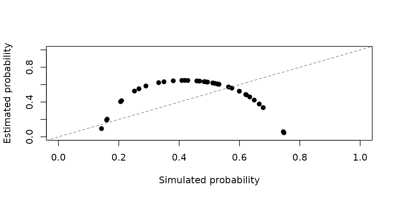

The example examines one fitted dataset. It does not establish accuracy across signal families or high-dimensional predictor distributions.