Order-2 logistic trend filtering: synthetic truth and held-out prediction

A binary response gives a zero or one at each observation, but the quantity we want to estimate is a probability curve. Here we fit

$$Y_i\mid x_i\sim\operatorname{Bernoulli}(p(x_i)),\qquad \operatorname{logit}p(x)=f(x).$$

Order 2 means piecewise quadratic on the logit scale. The absolute-value penalty on third divided differences lets different parts of the curve have different amounts of curvature. A large penalty removes adaptive knots and approaches a quadratic logit curve. It does not force a linear logit curve. Conversely, ordinary linear logistic regression already gives a curved, S-shaped probability response; that shape alone is not evidence of a nonlinear logit relationship.

This vignette first uses known synthetic probabilities, then the published Pima training/test data in MASS. We compare a constant probability, a linear logit, a quadratic logit, a natural-spline logit and trend filtering. All tuning uses training outcomes only. Separate test outcomes assess probability prediction; training fit is not used as evidence of predictive improvement.

A complete fit and a clear validation boundary

Supply a penalty path explicitly. lambda refers to predictor locations normalized to the training range, so it is not expressed in the original units of x. The default lambda.selection="fixed" returns a path without selecting one member. To select by minimum cross-validated log loss, supply training-fold labels:

make_folds <- function(y, k=5L, seed=1L) {
    set.seed(seed)
    fold <- integer(length(y))
    for (value in c(0, 1)) {
        at <- which(y == value)
        fold[at] <- sample(rep(seq_len(k), length.out=length(at)))
    }
    fold
}
log_loss <- function(y, eta) {
    mean((1-y)*pmax(eta, 0) + y*pmax(-eta, 0) +
         log1p(exp(-abs(eta))))
}
probability_scores <- function(y, eta, truth=NULL) {
    p <- plogis(eta)
    c(`Log loss`=log_loss(y, eta), `Brier score`=mean((p-y)^2),
      `Probability RMSE`=if (is.null(truth)) NA_real_ else sqrt(mean((p-truth)^2)))
}
lambda_path <- c(Inf, 10^seq(0, -4, by=-0.5))
spline_df <- c(3L, 5L, 7L)

By default, cv.penalty.scale="training_mass" multiplies each fold’s lambda and explicit ridge coefficients by its training/full weight-sum ratio. The fitting loss is a sum, so this preserves the penalty coefficient relative to mean loss. For example, four-fifths of the observations with unit weights use four-fifths of the reference penalty. The selected full-data fit uses the original supplied penalty. cv.penalty.scale="none" reproduces the earlier unchanged-numerical-penalty convention. Training ranges and covariate transformations are still recomputed within folds. Inspect cv.fold.lambda, cv.fold.penalty.factors, and cv.fold.ridge to see the actual fold settings.

The examples have independent observations, so the five folds are stratified by training outcome and assigned at the observation level. Repeated specimens from one person should instead share a fold label. Splitting must reflect the unit that will be held out in the intended application.

Log loss uses natural logarithms and evaluates the predicted probability of the observed outcome. The Brier score is squared probability error against the binary response. Both are lower-is-better prediction losses. Synthetic examples also allow probability RMSE against the known generating curve; this measure is unavailable for the real data.

Reusable fitting and plotting helpers are printed in the appendix. They learn predictor normalization, spline knots and covariate scaling within each training fold. The natural spline selects 3, 5 or 7 degrees of freedom using the same folds and loss as trend filtering. Constant, linear and quadratic logit models have no tuning parameter. All models use zero additional ridge in the comparisons below.

Recover known probability curves

Both examples use 600 training observations and 2,000 independently drawn test observations. Locations are uniform on [0,1]. The formulas below specify the true log odds before any observations are generated or models compared:

Example	True log odds	Purpose
Linear logit	-2 + 4*x	Ordinary linear logistic regression is correctly specified.
Local changes	-1.4 + 2.8*exp(-((x-.35)/.08)^2) - 1.5*exp(-((x-.75)/.15)^2)	A narrow peak and broader trough require locally varying curvature.

truth_eta <- list(
    `Linear logit`=function(x) -2+4*x,
    `Local changes`=function(x) -1.4+2.8*exp(-((x-.35)/.08)^2)-
        1.5*exp(-((x-.75)/.15)^2))
synthetic <- vector("list", length(truth_eta)); names(synthetic) <- names(truth_eta)
for (j in seq_along(truth_eta)) {
    set.seed(9100L+j)
    train_x <- runif(600); train_p <- plogis(truth_eta[[j]](train_x))
    train_y <- rbinom(600, 1, train_p)
    test_x <- runif(2000); test_p <- plogis(truth_eta[[j]](test_x))
    test_y <- rbinom(2000, 1, test_p)
    folds <- make_folds(train_y, seed=110L+j)
    fit <- fit_comparison(train_x, train_y, folds)
    synthetic[[j]] <- list(x=train_x, y=train_y, test_x=test_x,
        test_y=test_y, test_p=test_p, folds=folds, fit=fit)
}
knitr::kable(do.call(rbind, lapply(names(synthetic), function(name) {
    d <- synthetic[[name]]
    data.frame(Example=name, `Training observations`=length(d$y),
        `Training events`=sum(d$y), `Test observations`=length(d$test_y),
        `Test events`=sum(d$test_y), check.names=FALSE)
})), row.names=FALSE)

Example	Training observations	Training events	Test observations	Test events
Linear logit	600	300	2000	1008
Local changes	600	149	2000	481

Here is the public fit call for the local-changes example. Every candidate is refitted on each training fold, and all normalization is learned within that fold. No test outcomes enter this call:

d <- synthetic[["Local changes"]]
fit <- fit.logistic.trend.filtering(d$x, d$y, lambda=lambda_path,
    lambda.selection="cv", foldid=d$folds, backend="banded")
fit$cv.table
fit$diagnostics
predict(fit, seq(0, 1, length.out=300))

grid <- seq(0,1,length.out=300)
old_par <- par(mfrow=c(1,2), mar=c(4,4,2.5,.5))
for (name in names(synthetic)) {
    d <- synthetic[[name]]
    curve_plot(d$x, d$y, grid, predict_comparison(d$fit, grid),
               name, truth=plogis(truth_eta[[name]](grid)))
}

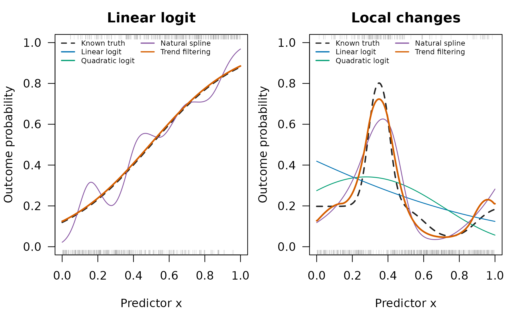
Known probabilities and training-data fits. Bottom rugs show controls and top rugs show events. Both panels use the same probability scale; separate test observations assess prediction below.

par(old_par)

Inspect the penalty choice, not just the final curve

The dashed horizontal line is the CV loss of the quadratic limit. The dotted vertical line marks the selected finite penalty when there is one. CV losses are training-fold averages, not test performance estimates or confidence intervals. Small numerical differences among strongly smoothed candidates need not correspond to different curve shapes; the adaptive-knot count helps show whether the fitted curve actually departed from the quadratic span.

old_par <- par(mfrow=c(1,2), mar=c(4,4,2.5,.5))
for (name in names(synthetic)) cv_plot(synthetic[[name]]$fit, name)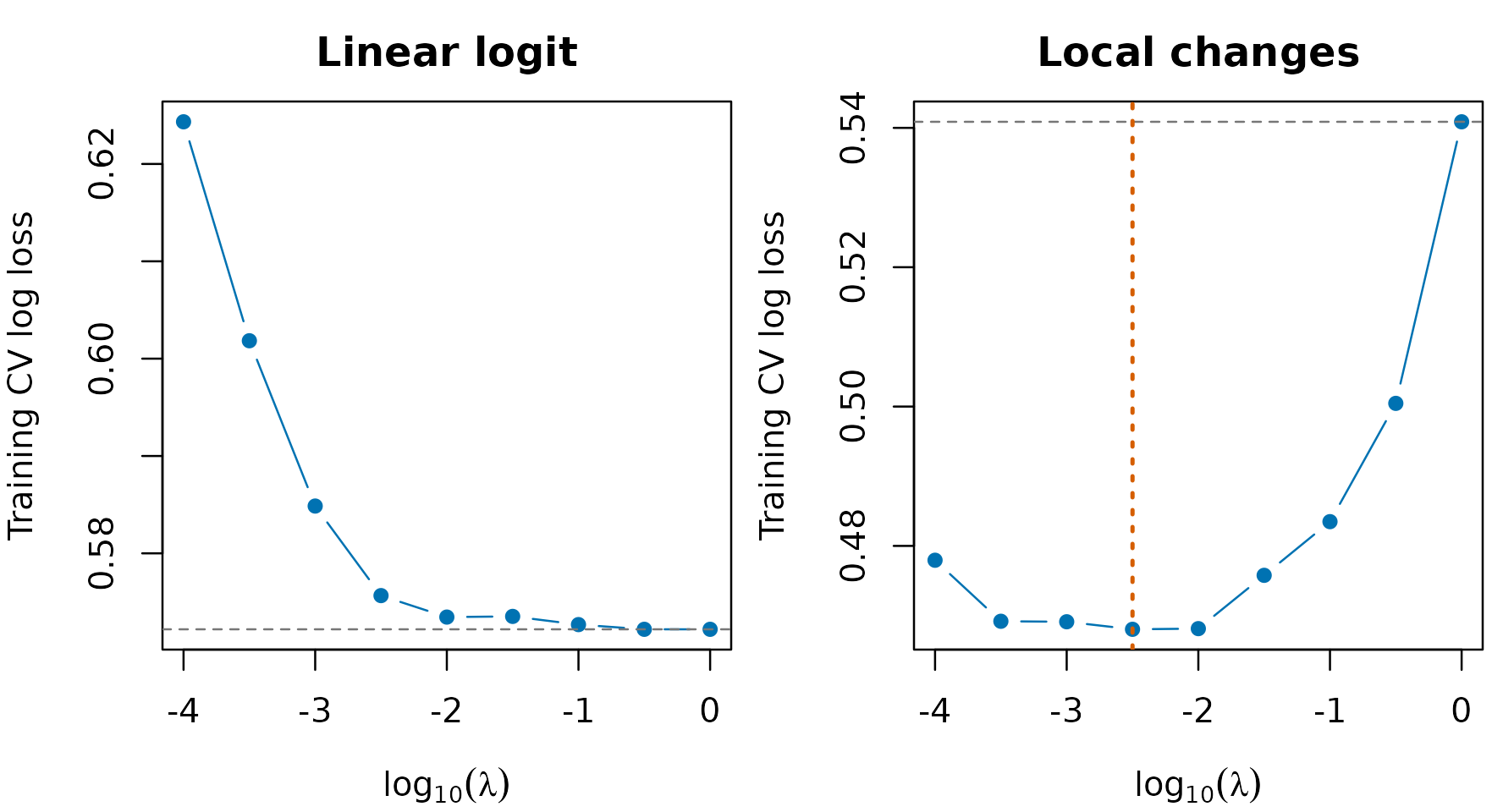

Training-only penalty selection on the same five folds used by the spline comparator. Blue points show finite penalties, the gray dashed line the quadratic limit, and an orange dotted line the selected finite penalty. The quadratic limit cannot be placed on a log10(lambda) axis.

par(old_par)
knitr::kable(do.call(rbind, lapply(names(synthetic), function(name)
    cbind(Example=name, tuning_summary(synthetic[[name]]$fit)))), row.names=FALSE)

Example	Selected lambda	Adaptive knots	Eligible lambda candidates	Lambda candidates	Selected spline df
Linear logit	Quadratic limit	0	10	10	7
Local changes	3.16e-03	6	10	10	5

A minimum at the smallest supplied penalty can signal a grid boundary; it is not evidence that still weaker penalties would help. Report that condition and investigate using training data in a separate analysis. The grid here is fixed in advance and is not extended in response to test results.

Strong, selected and weak smoothing

d <- synthetic[["Local changes"]]; tf <- d$fit$tf
indices <- c(which(is.infinite(tf$lambda)), tf$selected.index, which.min(tf$lambda))
path_p <- plogis(predict(tf, grid, lambda.index=indices, type="link"))
old_par <- par(mar=c(4,4,1,.5))
plot(grid, plogis(truth_eta[["Local changes"]](grid)), type="l", ylim=c(0,1),
     xlab="Predictor x", ylab="Outcome probability", lwd=2, lty=2, col="#222222")
matlines(grid, path_p, col=c("#009E73", "#D55E00", "#0072B2"), lty=c(1,1,3), lwd=2)
legend("topright", c("Known truth", "Quadratic limit", "Selected penalty", "Weakest penalty"),
       col=c("#222222", "#009E73", "#D55E00", "#0072B2"), lty=c(2,1,1,3), bty="n", cex=.8)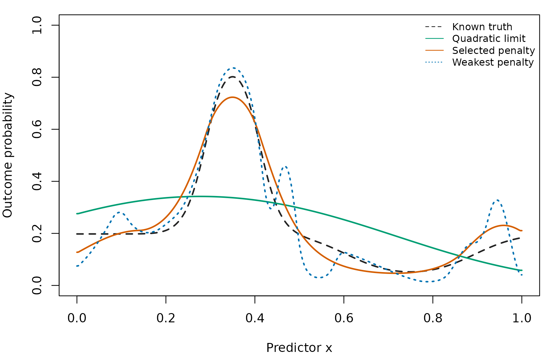

Three members of the same local-changes path: the quadratic limit, the CV-selected candidate, and the weakest supplied penalty. Coincident curves are retained when the selected candidate is an endpoint.

par(old_par)

synthetic_scores <- do.call(rbind, lapply(names(synthetic), function(name) {
    d <- synthetic[[name]]
    cbind(Example=name, score_comparison(d$fit, d$test_x, d$test_y, d$test_p))
}))
knitr::kable(synthetic_scores, digits=4, row.names=FALSE)

Example	Model	Log loss	Brier score	Probability RMSE
Linear logit	Constant probability	0.6931	0.2500	0.2427
Linear logit	Linear logit	0.5523	0.1849	0.0067
Linear logit	Quadratic logit	0.5523	0.1849	0.0066
Linear logit	Natural spline	0.5657	0.1889	0.0599
Linear logit	Trend filtering	0.5523	0.1849	0.0066
Local changes	Constant probability	0.5518	0.1827	0.1991
Local changes	Linear logit	0.5365	0.1782	0.1868
Local changes	Quadratic logit	0.5266	0.1722	0.1650
Local changes	Natural spline	0.4847	0.1557	0.0808
Local changes	Trend filtering	0.4757	0.1523	0.0457

In the linear-logit example, trend filtering selected 0 adaptive knots. Its probability RMSE is 0.0066, compared with 0.0067 for the correctly specified linear logit model. The spline’s extra flexibility in this draw does not improve its independent test predictions.

For the local-changes signal, trend filtering selected 6 adaptive knots and has probability RMSE 0.0457, compared with 0.1868 for linear logistic regression. This is the intended contrast between a simple logit relationship and a locally changing one.

The probability-RMSE column compares each prediction with the generating probability at the same test location. Log loss and Brier score also include binary sampling variation. These two fixed examples illustrate possible behaviors, including extra flexibility when the linear model is correct. They are not a repeated-simulation ranking or a claim that trend filtering always wins. Predictions outside the training range are included: trend filtering holds its boundary curve value, while the reference models extrapolate their specified functions.

Exact ties and binomial trial weights

Repeated values of x share a curve value. When no covariates or offsets differ within a group, independent binary trials can equivalently be represented by a success proportion and trial count. This is an equality of likelihoods, not a reason to bin distinct predictor values.

set.seed(9140)
x_group <- seq(0,1,length.out=12)
trials <- rep(c(8L, 12L, 16L), 4)
successes <- rbinom(length(x_group), trials, plogis(-1+2*x_group))
x_individual <- rep(x_group, trials)
y_individual <- unlist(Map(function(s, n) c(rep(1, s), rep(0, n-s)), successes, trials))
individual <- fit.logistic.trend.filtering(x_individual, y_individual,
    lambda=.01, backend="banded")
grouped <- fit.logistic.trend.filtering(x_group, successes/trials,
    weights=trials, lambda=.01, backend="banded")
maximum_difference <- max(abs(as.numeric(predict(individual, grid))-
                              as.numeric(predict(grouped, grid))))
stopifnot(maximum_difference < 1e-7,
          abs(individual$fits[[1]]$objective-grouped$fits[[1]]$objective) < 1e-6)
knitr::kable(data.frame(`Binary records`=length(y_individual),
    `Distinct locations`=length(x_group), `Maximum probability difference`=maximum_difference,
    check.names=FALSE), digits=9)

Binary records	Distinct locations	Maximum probability difference
144	12	0

The fixed penalty makes this a direct numerical equivalence check, not a prediction comparison. Do not collapse records merely because x is tied if their covariates or offsets differ. The ordinary record-level interface retains those contributions separately.

Pima data: fit on training women, assess on test women

MASS::Pima.tr and MASS::Pima.te contain a published random split of 532 complete records into 200 training and 332 test subjects. The population was women of Pima heritage, aged at least 21, living near Phoenix, Arizona; diabetes status was determined according to WHO criteria. These examples classify the recorded diabetes status, not future disease onset or a causal glucose effect. See the MASS dataset documentation for provenance and variable definitions. This complete-record subset does not represent all patients or resolve the original missing-data selection.

Glucose is the sole nonlinear predictor. We retain its recorded dataset scale; the MASS help describes the measurement but does not specify its units. No outcome-dependent transformation, feature screening or new train/test split is introduced.

pima_train <- MASS::Pima.tr
pima_y <- as.numeric(pima_train$type == "Yes")
pima_folds <- make_folds(pima_y, seed=9201)
pima <- fit_comparison(pima_train$glu, pima_y, pima_folds)
# Freeze the predeclared optional adjusted comparison before opening the test set.
z_train <- as.matrix(pima_train[, c("age", "bmi")])
pima_adjusted <- fit_comparison(pima_train$glu, pima_y, pima_folds,
                               covariates=z_train)
knitr::kable(tuning_summary(pima), row.names=FALSE)

Selected lambda	Adaptive knots	Eligible lambda candidates	Lambda candidates	Selected spline df
Quadratic limit	0	10	10	3

All selection above used only the 200 training women. Candidate eligibility is explicit: a trend-filtering candidate must pass every training fold and the full training fit. A spline candidate must have converged without fitting warnings on every fold; any failed candidate has an unavailable CV loss. The quadratic-limit and all finite candidates remain visible:

pima_cv <- pima$tf$cv.table
pima_cv$lambda <- vapply(pima_cv$lambda, penalty_label, character(1))
pima_cv$selected <- seq_len(nrow(pima_cv)) == pima$tf$selected.index
pima_cv$full.fit.status <- pima$tf$diagnostics$status
knitr::kable(pima_cv, digits=4, row.names=FALSE)

lambda	log.loss	eligible	selected	full.fit.status
Quadratic limit	0.5276	TRUE	TRUE	converged
1e+00	0.5276	TRUE	FALSE	converged
3.16e-01	0.5276	TRUE	FALSE	converged
1e-01	0.5276	TRUE	FALSE	converged
3.16e-02	0.5276	TRUE	FALSE	converged
1e-02	0.5315	TRUE	FALSE	converged
3.16e-03	0.5405	TRUE	FALSE	converged
1e-03	0.5482	TRUE	FALSE	converged
3.16e-04	0.5627	TRUE	FALSE	converged
1e-04	0.6404	TRUE	FALSE	converged

knitr::kable(pima$spline_cv, digits=4, row.names=FALSE)

df	log.loss	eligible
3	0.5319	TRUE
5	0.5450	TRUE
7	0.5578	TRUE

The selected Pima trend-filtering fit has 0 adaptive knots. Here the strongly smoothed candidates have virtually identical CV losses; the selected finite penalty still gives a quadratic logit curve. Numerical differences on a flat part of the CV path should not be interpreted as support for additional complexity.

Only now load and score the published test set. It is never passed to a tuning or fitting function. The optional adjustment analysis later follows the same training-only rule.

pima_test <- MASS::Pima.te
pima_test_y <- as.numeric(pima_test$type == "Yes")
pima_eta <- predict_comparison(pima, pima_test$glu)
pima_scores <- score_comparison(pima, pima_test$glu, pima_test_y)
knitr::kable(data.frame(Split=c("Training", "Test"),
    Women=c(nrow(pima_train), nrow(pima_test)),
    Events=c(sum(pima_y), sum(pima_test_y)),
    `Glucose minimum`=c(min(pima_train$glu), min(pima_test$glu)),
    `Glucose maximum`=c(max(pima_train$glu), max(pima_test$glu)), check.names=FALSE))

Split	Women	Events	Glucose minimum	Glucose maximum
Training	200	68	56	199
Test	332	109	65	197

knitr::kable(pima_scores[, c("Model", "Log loss", "Brier score")], digits=4, row.names=FALSE)

Model	Log loss	Brier score
Constant probability	0.6333	0.2207
Linear logit	0.4938	0.1603
Quadratic logit	0.4967	0.1614
Natural spline	0.4973	0.1617
Trend filtering	0.4967	0.1614

pima_outside <- sum(pima_test$glu < min(pima_train$glu) |
                    pima_test$glu > max(pima_train$glu))

On these 332 test women, trend filtering has log loss 0.4967, compared with 0.4938 for linear logistic regression. Thus the flexible method does not improve on the linear comparator in this example. The difference is small and one split does not establish general superiority of either method.

There are 0 test women outside the training glucose range. All 332 test women remain in the score table. Different boundary/extrapolation rules can matter there; those rows are not silently discarded.

pima_grid <- seq(min(pima_train$glu), max(pima_train$glu), length.out=250)
old_par <- par(mar=c(4,4,2.5,.5))
curve_plot(pima_train$glu, pima_y, pima_grid,
           predict_comparison(pima, pima_grid), "Diabetes status and glucose",
           xlab="Plasma glucose (recorded dataset scale)")
bins <- bin_summary(pima_train$glu, pima_y)
segments(bins$x, bins$lower, bins$x, bins$upper, col="#555555")
points(bins$x, bins$observed, pch=21, bg="white", cex=.9)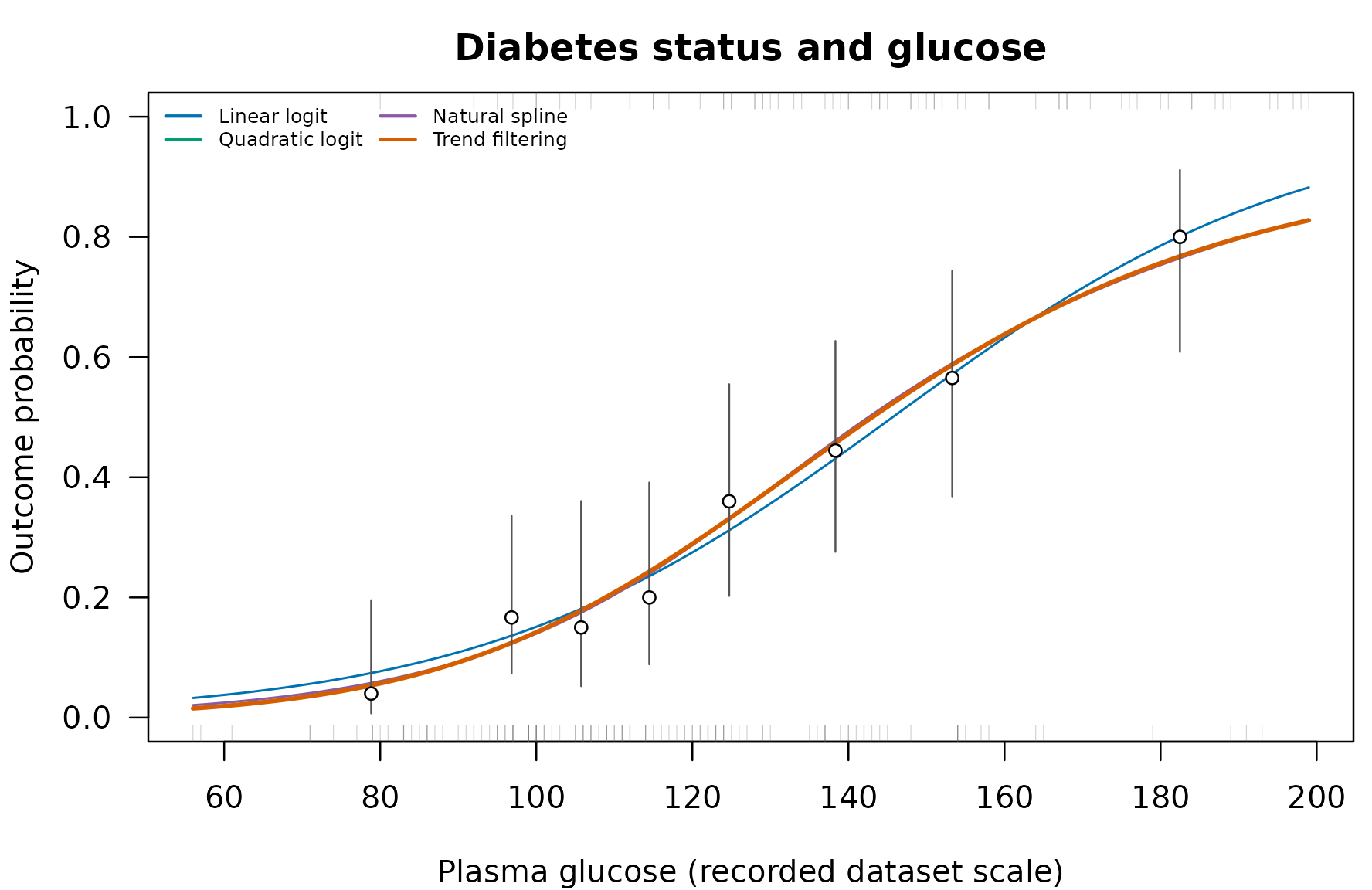

Training-data fits and descriptive training proportions. Points and 95% Wilson intervals summarize glucose groups; they are not confidence bands for a fitted curve. Bottom/top rugs mark training controls/events. Models used every original training record, without binning.

par(old_par)

Check calibration as well as average loss

Calibration asks whether predicted probabilities match observed frequencies. The plot groups held-out predictions into approximately equal-sized groups and compares their mean prediction with observed event proportions. The intervals describe those groups, not uncertainty in a selected trend-filtering curve. No test-derived calibration correction is applied to the reported scores.

old_par <- par(pty="s")
plot(c(0,1), c(0,1), type="n", xlab="Mean predicted probability",
     ylab="Observed test event proportion", xlim=c(0,1), ylim=c(0,1),
     xaxs="i", yaxs="i")
abline(0,1,lty=2,col="#777777")
for (name in c("Linear logit", "Trend filtering")) {
    b <- bin_summary(plogis(pima_eta[, name]), pima_test_y, bins=5)
    color <- curve_colors[name]
    segments(b$x, b$lower, b$x, b$upper, col=color)
    points(b$x, b$observed, col=color, pch=if (name=="Linear logit") 16 else 17)
}
legend("topleft", c("Linear logit", "Trend filtering"),
       col=curve_colors[c("Linear logit", "Trend filtering")], pch=c(16,17), bty="n")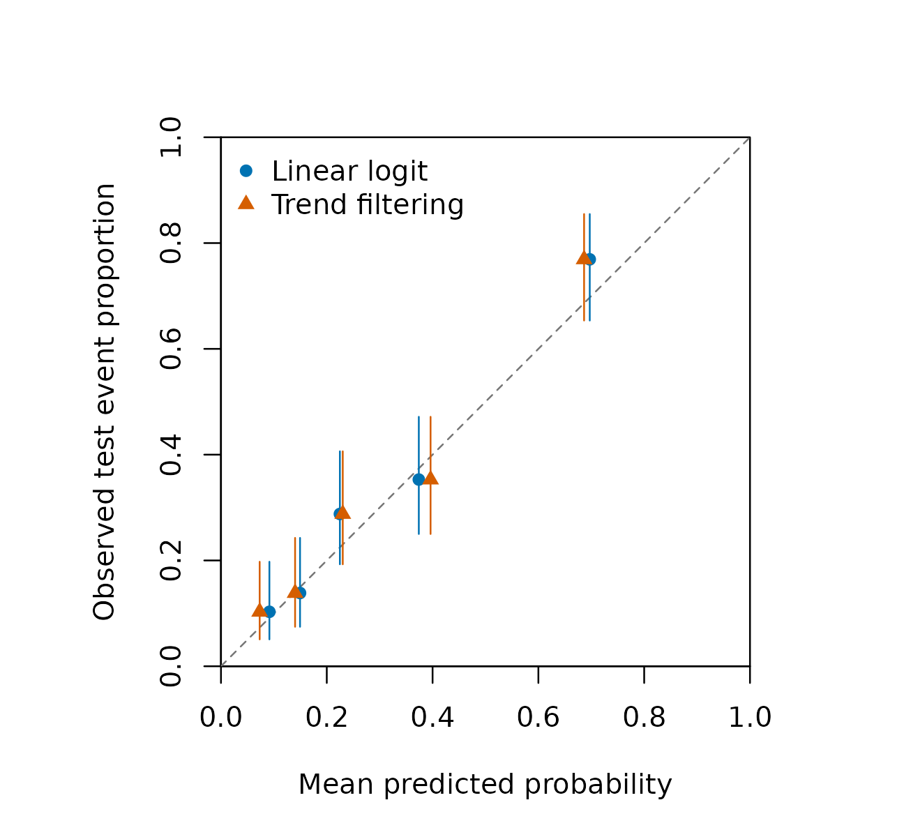

Calibration on the untouched 332-woman test set. Each model forms its own groups from predicted probabilities. The dashed diagonal is perfect agreement; intervals are descriptive 95% Wilson intervals.

par(old_par)
calibration <- do.call(rbind, lapply(c("Linear logit", "Trend filtering"), function(name) {
    eta <- pima_eta[, name]
    fit <- stats::glm(pima_test_y ~ eta, family=stats::binomial())
    stopifnot(fit$converged, all(is.finite(stats::coef(fit))))
    data.frame(Model=name, Intercept=unname(stats::coef(fit)[1]),
               Slope=unname(stats::coef(fit)[2]))
}))
knitr::kable(calibration, digits=3, row.names=FALSE)

Model	Intercept	Slope
Linear logit	0.232	1.123
Trend filtering	0.202	1.070

The intercept and slope come from a separate test-set logistic regression of the outcome on the predicted log odds. Ideal values are zero and one. They are descriptive checks on a modest test sample, not precise population parameters or evidence that any method is clinically validated. Small differences in one test split do not establish a general ordering of methods.

Optional age and BMI adjustment

A one-dimensional nonlinear curve can be combined with additional linear covariates. We predeclare age and BMI here; they are not selected by looking at test losses. Their centering and scaling are learned within each training fold. All models in this comparison use the same covariates and zero additional ridge.

z_test <- as.matrix(pima_test[, c("age", "bmi")])
adjusted_scores <- score_comparison(pima_adjusted, pima_test$glu, pima_test_y,
                                   covariates=z_test)
show_adjusted <- adjusted_scores$Model %in% c("Linear logit", "Quadratic logit", "Trend filtering")
knitr::kable(adjusted_scores[show_adjusted, c("Model", "Log loss", "Brier score")],
             digits=4, row.names=FALSE)

Model	Log loss	Brier score
Linear logit	0.4535	0.1473
Quadratic logit	0.4553	0.1483
Trend filtering	0.4553	0.1483

knitr::kable(tuning_summary(pima_adjusted), row.names=FALSE)

Selected lambda	Adaptive knots	Eligible lambda candidates	Lambda candidates	Selected spline df
Quadratic limit	0	10	10	3

profile <- apply(z_train, 2, stats::median)

For the following conditional curves, age is fixed at the training median of 28 years and BMI at 32.8 kg/m^2. Test scores above use each test woman’s own age and BMI; the median profile is only a plotting reference.

z_grid <- matrix(rep(profile, each=length(pima_grid)), ncol=2,
                 dimnames=list(NULL, colnames(z_train)))
old_par <- par(mfrow=c(1,2), mar=c(4,4,2.5,.5))
curve_plot(pima_train$glu, pima_y, pima_grid, predict_comparison(pima, pima_grid),
           "Glucose only", xlab="Glucose (recorded scale)")
curve_plot(pima_train$glu, pima_y, pima_grid,
           predict_comparison(pima_adjusted, pima_grid, z_grid),
           "Adjusted, median profile", xlab="Glucose (recorded scale)")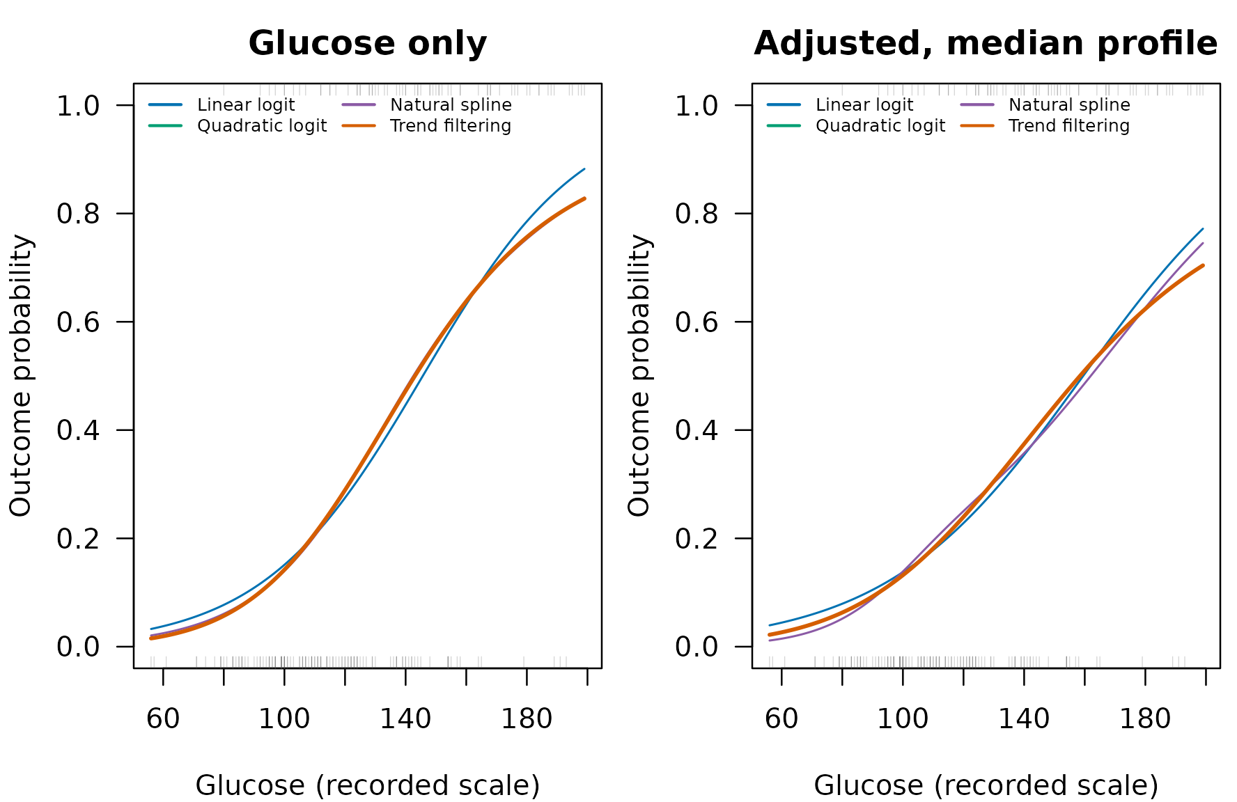

Conditional probability curves with age and BMI fixed at their training medians. The adjustment changes the question; these curves are neither population averages nor causal effects. Sparse support for particular glucose/age/BMI combinations remains possible.

par(old_par)

Adjustment does not make the glucose curve causal. A selected knot or a visually striking bend is not automatically a biological threshold. Plotting many candidate markers and choosing an attractive curve would require a separate selection and validation strategy.

Convergence, boundaries and larger samples

The selected fit must pass its numerical diagnostics. Stationarity measures remaining violations of the objective’s first-order conditions; dual feasibility and complementarity check the L1 penalty conditions. These are numerical checks, not evidence of statistical validity or a proof that every logistic problem has a finite minimizer.

selected_diagnostics <- do.call(rbind, lapply(
    list(`Synthetic linear`=synthetic[[1]]$fit,
         `Synthetic local changes`=synthetic[[2]]$fit,
         `Pima glucose`=pima, `Pima adjusted`=pima_adjusted), function(object) {
        object$tf$diagnostics[object$tf$selected.index,
            c("lambda", "converged", "status", "stationarity", "complementarity", "backend", "working.knots")]
    }))
diagnostic_table <- data.frame(
    Example=rownames(selected_diagnostics),
    Lambda=vapply(selected_diagnostics$lambda, penalty_label, character(1)),
    Converged=selected_diagnostics$converged,
    Stationarity=formatC(selected_diagnostics$stationarity, format="e", digits=2),
    Complementarity=formatC(selected_diagnostics$complementarity, format="e", digits=2),
    Knots=selected_diagnostics$working.knots)
knitr::kable(diagnostic_table, row.names=FALSE)

Example	Lambda	Converged	Stationarity	Complementarity	Knots
Synthetic linear	Quadratic limit	TRUE	1.30e-10	0.00e+00	0
Synthetic local changes	3.16e-03	TRUE	2.33e-10	0.00e+00	6
Pima glucose	Quadratic limit	TRUE	2.63e-12	0.00e+00	0
Pima adjusted	Quadratic limit	TRUE	2.76e-11	0.00e+00	0

stopifnot(all(selected_diagnostics$converged))

A failure is not repaired by treating its fitted probabilities as valid:

failed <- fit.logistic.trend.filtering(synthetic[[2]]$x, synthetic[[2]]$y,
    lambda=.001, backend="banded", control=list(max.iterations=1L), warn=FALSE)
failed$diagnostics[, c("converged", "status")]
#>   converged          status
#> 1     FALSE iteration_limit
stopifnot(!failed$diagnostics$converged, all(is.na(predict(failed))))

Inspect failed candidate/fold status before changing iteration budgets or numerical settings. Separation may prevent a finite fit; adding ridge changes the objective and must be reported. Predictor values outside the training range receive the boundary curve value. When covariates or offsets are present, their contributions still vary normally.

backend="banded" avoids full observation-by-knot dense matrices in fitting and prediction while checking all original knot coefficients. backend="auto" uses it above 256 distinct values or when the dense workspace estimate exceeds its guard. backend="dense" remains a small-problem reference. Thousands of observations do not change the fact that the nonlinear component is one-dimensional.

For an optional scaling check, increase n in the following code. It is not run during routine vignette builds, and no hardware-specific timing claim is made here:

set.seed(9301)
n <- 24000L
x <- runif(n)
y <- rbinom(n, 1, plogis(-1+sin(6*pi*x)))
system.time(large_fit <- fit.logistic.trend.filtering(x, y,
    lambda=c(1, .1, .01, .001), backend="banded"))
large_fit$diagnostics

The classical minimax-rate result concerns appropriately tuned Gaussian trend filtering over specified function classes. It does not automatically establish optimality for this logistic model, covariate adjustment or a selected real-data curve. This vignette supports reproducible fitting and assessment, not a claim of universal superiority. No confidence band is supplied that would ignore penalty and knot selection.

Does the probability vary with the predictor?

The global question is whether all observed predictor locations share one unknown binary probability. The null estimate is the sample event rate. This differs from asking where the curve departs from a constant, and rejecting constancy does not by itself establish nonlinearity: linear logistic regression can also describe a nonconstant probability.

assess.logistic.trend.filtering() takes a fitted object and performs two separate assessments. It retunes the supplied, prespecified penalty path on new outcome-independent folds, then repeats this complete procedure after each outcome permutation. Its default statistic is twice the ordinary binomial log-likelihood improvement over the constant, truncated at zero for numerical roundoff. The returned fit is this newly tuned fit; the input object’s fold labels and selected penalty are not reused. This avoids conditioning on folds that may have been stratified using the observed outcomes.

Separately, nested CV estimates prediction loss: outer test outcomes enter neither penalty selection nor the outer-training event rate used as the constant baseline. Improvement means constant loss minus smoother loss. Positive values favor the smoother. These are predictive assessment scores, not confidence intervals or a second significance test.

The following fixed examples use independent binary observations without covariates, offsets or weights. One has constant probability 0.35; the other has a localized probability peak. The predictor, penalty path and all solver settings are specified before generating outcomes. There are 160 observations per example. We use 99 permutations to keep routine builds short, giving p-value resolution 0.01; the assessment function defaults to 999. These two examples illustrate the outputs, not average false-positive rates or power. We also prespecify the two optional shape tests below; all three tests share the same fitted models and permutations.

assessment_examples <- list()
for (j in 1:2) {
    set.seed(9400L+j)
    x <- seq(0, 1, length.out=160)
    probability <- if (j == 1) rep(.35, length(x)) else
        plogis(-2+4.8*exp(-((x-.4)/.15)^2))
    y <- rbinom(length(x), 1, probability)
    fit <- fit.logistic.trend.filtering(x, y, lambda=c(Inf, .1, .01, .001),
                                       backend="banded")
    assessment_examples[[j]] <- assess.logistic.trend.filtering(fit,
        permutations=99, inner.folds=3, outer.folds=5, seed=9500L+j,
        additional.tests=c("absolute.deviation", "total.variation"))
}
names(assessment_examples) <- c("Constant truth", "Localized peak")
assessment_scores <- do.call(rbind, lapply(names(assessment_examples), function(name) {
    a <- assessment_examples[[name]]
    stopifnot(a$status == "complete", a$prediction$status == "complete")
    data.frame(Example=name, `Permutation p-value`=a$p.value,
        `Log-loss improvement`=unname(a$prediction$improvement["log.loss"]),
        `Brier improvement`=unname(a$prediction$improvement["brier"]), check.names=FALSE)
}))
knitr::kable(assessment_scores, row.names=FALSE, digits=4)

Example	Permutation p-value	Log-loss improvement	Brier improvement
Constant truth	0.91	-0.0087	-0.0038
Localized peak	0.01	0.1434	0.0761

The constant-truth example has permutation p-value 0.91 and nested-CV log-loss improvement -0.0087. The localized-peak example has p-value 0.01 and log-loss improvement 0.1434. The p-value measures evidence against constancy under exchangeability; the prediction gain measures whether that pattern helps on held-out observations.

How large is the fitted departure from constancy?

Every assessment returns curve.summaries, even when only the default likelihood test is requested. With fitted probabilities $\hat p(x_i)$ and sample event rate $\bar y$, absolute deviation is

$$\delta_0 = \frac{1}{n}\sum_{i=1}^n |\hat p(x_i)-\bar y|.$$

This averages over participants, including multiple participants at the same predictor value. It does not give equal weight to sparsely and densely sampled parts of a uniformly spaced grid. For example, $\delta_0=0.04$ means an average absolute probability difference of four percentage points. It summarizes the fitted curve; sampling noise and smoothing bias still affect it.

Total variation measures accumulated rises and falls across the entire observed predictor range. Let $s_1,\ldots,s_K$ be the ordered endpoints, knots and interior turning points of the fitted curve. Then

$$\delta_1 = \sum_{j=2}^K |\hat p(s_j)-\hat p(s_{j-1})|.$$

The logit is quadratic between knots, so its interior turning points can be located algebraically. The implementation evaluates each segment’s endpoints and midpoint to recover that quadratic in local coordinates. Since the logistic transformation is monotone, the probability curve has the same turning points. This avoids missing an interior peak on a coarse grid. A monotone curve’s total variation equals its absolute endpoint difference; several rises and falls can accumulate to a value above one. Total variation is sensitive to small oscillations and is distinct from the order-2 penalty.

shape_scores <- do.call(rbind, lapply(names(assessment_examples), function(name) {
    a <- assessment_examples[[name]]
    data.frame(Example=name,
        `Mean absolute deviation`=unname(a$curve.summaries["absolute.deviation"]),
        `Total variation`=unname(a$curve.summaries["total.variation"]),
        check.names=FALSE)
}))
knitr::kable(shape_scores, row.names=FALSE, digits=4)

Example	Mean absolute deviation	Total variation
Constant truth	0.0221	0.1677
Localized peak	0.2615	1.5857

The additional.tests argument requests permutation tests for either or both summaries. Each shuffle repeats tuning exactly as for likelihood, then computes the requested summaries from that selected fit. Larger values are compared with the permutation distribution using inclusive exceedances and the same plus-one p-value rule. This adds curve evaluation but no extra model fits. No t-test is applied to simulated bootstrap or permutation differences.

shape_tests <- do.call(rbind, lapply(names(assessment_examples), function(name) {
    tt <- assessment_examples[[name]]$tests
    stopifnot(all(tt$status == "complete"))
    data.frame(Example=name, Statistic=tt$test,
        `Individual p-value`=tt$p.value, `Holm p-value`=tt$p.value.holm,
        check.names=FALSE)
}))
knitr::kable(shape_tests, row.names=FALSE, digits=3)

Example	Statistic	Individual p-value	Holm p-value
Constant truth	likelihood	0.91	1.00
Constant truth	absolute.deviation	0.90	1.00
Constant truth	total.variation	0.73	1.00
Localized peak	likelihood	0.01	0.03
Localized peak	absolute.deviation	0.01	0.03
Localized peak	total.variation	0.03	0.03

The Holm column adjusts across the three statistics within each assessment. It does not adjust across the two examples or a wider family of outcomes and phylotypes. The scalar p.value remains the individual likelihood p-value for backward compatibility. Prespecify the tests; choosing the smallest individual p-value after inspecting the table would ignore multiple testing. These examples do not establish that one statistic has greater power than another.

old_par <- par(mfrow=c(1, 2), mar=c(4, 4, 2, .5))
for (name in names(assessment_examples)) {
    a <- assessment_examples[[name]]
    hist(a$permutations$statistic, breaks=10, col="grey85", border="white",
         xlim=range(c(0, a$statistic, a$permutations$statistic)), main=name,
         xlab="Likelihood improvement statistic", ylab="Permutation count")
    abline(v=a$statistic, col="#D55E00", lwd=2)
}

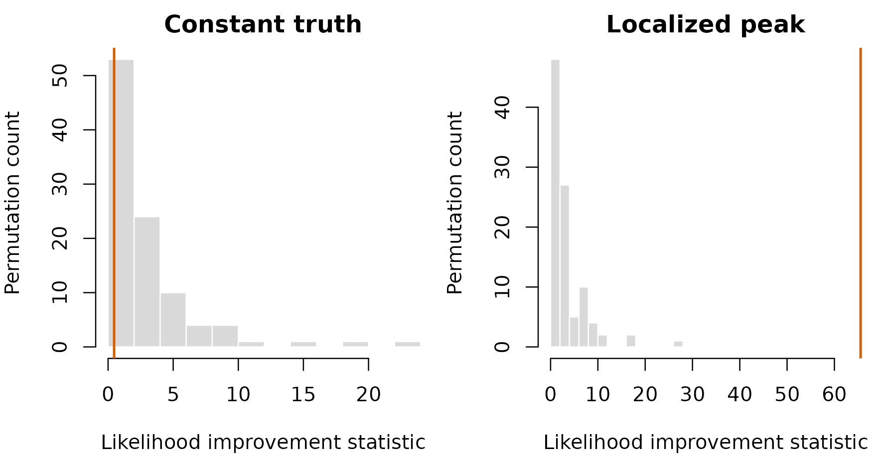
Each histogram shows likelihood improvements after randomly shuffling outcomes while retaining predictor locations and the event count. The orange line marks the observed statistic. The horizontal scales include the observed statistic, so an unusually large improvement can lie far beyond the shuffled results.

par(old_par)

Inspect assessment$permutations, assessment$permutation.diagnostics and assessment$prediction$diagnostics for numerical failures. If any permutation cannot select a valid fit, p.value is unavailable; p.value.bounds shows the range obtained by counting each missing statistic at either extreme. That range is not a confidence interval. Incomplete outer predictions similarly leave the smoother’s overall prediction scores unavailable. Failed fits are not dropped and denominators are not reduced to successful replicates. For optional tests, inspect tests and permutation.statistics. Missing statistics leave the affected individual p-value unavailable, with lower and upper failure bounds. If any requested test is incomplete, the whole Holm column is unavailable. A curve-summary arithmetic failure is recorded in curve.summary.details or the corresponding permutation diagnostic; it does not erase an otherwise available likelihood statistic. Neither the summaries nor their tests provide pointwise or simultaneous confidence bands.

Unrestricted outcome shuffling is not valid for repeated participants, dependent observations or confounder-adjusted null hypotheses. The assessment rejects nonbinary responses, nonunit weights, covariates and offsets; callers must establish independence. A path or predictor chosen after inspecting outcomes is an additional selection step that this assessment does not repeat. This workflow uses an outcome permutation under the null, rather than a bootstrap intended to estimate uncertainty around the fitted alternative.

What would a 95% uncertainty band mean?

The current fitter returns point estimates and convergence diagnostics, not standard errors or posterior draws. The Wilson intervals in the Pima figures describe observed bin proportions; they are not confidence bands for the trend-filtering curve.

A pointwise 95% interval concerns the probability at one prespecified predictor value. A simultaneous 95% band aims to cover the entire curve over a specified domain; taking pointwise intervals at many locations does not produce such a band. A region average, contrast between regions, or location of an adaptive knot is another inferential target and needs its own uncertainty calculation.

One practical extension is a bootstrap of the complete fitting procedure, including penalty selection in each replicate. Independent observations may be resampled individually; repeated observations should be resampled by participant, and each participant’s copies must remain together in tuning folds. Binomial trial weights and any covariates or offsets must retain their sampling meaning. Failed fits and their frequency must be reported rather than silently dropped. Penalization bias and unstable knot selection can make ordinary bootstrap intervals miscalibrated. Before describing them as 95% confidence intervals, assess pointwise and simultaneous coverage separately on simulations with known truth, including sparse predictor regions, strong curvature and near-separation. A fixed-lambda bootstrap answers a different question from one that repeats tuning.

Bayesian credible intervals require an explicit probability model and priors, for example a binomial likelihood with shrinkage on third divided differences and proper priors on the unpenalized quadratic component and any covariates. Posterior sampling, smoothing-scale uncertainty and sampler diagnostics are additional work; optimizing the current penalized objective does not supply posterior draws. Bayesian trend filtering provides a precedent for binomial models. Its credible intervals express posterior uncertainty under the chosen model, without automatically guaranteeing 95% frequentist coverage. Likewise, the Gaussian generalized-lasso selective-inference results do not directly supply confidence bands for this cross-validated logistic fit.

Reusable analysis helpers

These helpers implement the comparisons and figures above. In particular, fit_reference() is called anew inside each spline-training fold; its stored model terms retain that fold’s spline knots for prediction.

method_names <- c("Constant probability", "Linear logit", "Quadratic logit",
                  "Natural spline", "Trend filtering")
curve_colors <- c("Linear logit"="#0072B2", "Quadratic logit"="#009E73",
                  "Natural spline"="#8B5AA5", "Trend filtering"="#D55E00")

fit_reference <- function(x, y, kind, df=NULL, covariates=NULL) {
    lo <- min(x); span <- diff(range(x))
    if (!is.finite(span) || span <= 0) stop("Training predictor needs a positive range.")
    d <- data.frame(y=y, u=(x-lo)/span)
    zcenter <- zscale <- numeric()
    if (!is.null(covariates)) {
        zcenter <- colMeans(covariates)
        zz <- sweep(covariates, 2, zcenter)
        zscale <- sqrt(colMeans(zz^2))
        if (any(zscale <= 0)) stop("Constant training covariate.")
        zz <- sweep(zz, 2, zscale, "/")
        for (j in seq_len(ncol(zz))) d[[paste0("z", j)]] <- zz[, j]
    }
    rhs <- switch(kind, constant="1", linear="u", quadratic="u + I(u^2)",
                  spline=sprintf("splines::ns(u, df=%d)", df))
    if (length(zcenter)) rhs <- paste(rhs, paste0("z", seq_along(zcenter), collapse=" + "), sep=" + ")
    messages <- character()
    fit <- withCallingHandlers(
        stats::glm(stats::as.formula(paste("y ~", rhs)), data=d,
                   family=stats::binomial(), control=stats::glm.control(maxit=100)),
        warning=function(w) {
            messages <<- c(messages, conditionMessage(w))
            invokeRestart("muffleWarning")
        })
    if (!fit$converged || any(!is.finite(stats::coef(fit))) || length(messages))
        stop(paste(c("Reference fit did not pass convergence checks.", messages), collapse=" "))
    list(model=fit, lo=lo, span=span, zcenter=zcenter, zscale=zscale)
}
predict_reference <- function(object, x, covariates=NULL) {
    d <- data.frame(u=(x-object$lo)/object$span)
    if (length(object$zcenter)) {
        zz <- sweep(sweep(covariates, 2, object$zcenter), 2, object$zscale, "/")
        for (j in seq_len(ncol(zz))) d[[paste0("z", j)]] <- zz[, j]
    }
    eta <- as.numeric(stats::predict(object$model, newdata=d, type="link"))
    if (any(!is.finite(eta))) stop("Nonfinite reference prediction.")
    eta
}
fit_comparison <- function(x, y, folds, covariates=NULL) {
    basic <- lapply(c("constant", "linear", "quadratic"), function(kind)
        fit_reference(x, y, kind, covariates=covariates))
    names(basic) <- method_names[1:3]
    losses <- matrix(NA_real_, max(folds), length(spline_df))
    spline_status <- matrix("complete", max(folds), length(spline_df))
    for (k in sort(unique(folds))) for (j in seq_along(spline_df)) {
        train <- folds != k; test <- !train
        ztrain <- if (is.null(covariates)) NULL else covariates[train, , drop=FALSE]
        ztest <- if (is.null(covariates)) NULL else covariates[test, , drop=FALSE]
        result <- tryCatch({
            fit <- fit_reference(x[train], y[train], "spline", spline_df[j], ztrain)
            log_loss(y[test], predict_reference(fit, x[test], ztest))*sum(test)
        }, error=function(e) e)
        if (inherits(result, "error")) spline_status[k, j] <- conditionMessage(result)
        else losses[k, j] <- result
    }
    cv_loss <- colSums(losses)/length(y)
    if (!any(is.finite(cv_loss))) stop("No spline candidate passed all training folds.")
    selected_df <- spline_df[which.min(replace(cv_loss, !is.finite(cv_loss), Inf))]
    spline <- fit_reference(x, y, "spline", selected_df, covariates)
    # Candidate failures are displayed in the diagnostic tables below.
    tf <- fit.logistic.trend.filtering(x, y, lambda=lambda_path,
        covariates=covariates, lambda.selection="cv", foldid=folds,
        backend="banded", warn=FALSE)
    if (is.null(tf$selected.index)) stop("No trend-filtering candidate passed every fold and the full fit.")
    list(basic=basic, spline=spline, tf=tf,
         spline_cv=data.frame(df=spline_df, log.loss=cv_loss,
                              eligible=is.finite(cv_loss)),
         spline_fold_status=spline_status)
}
predict_comparison <- function(object, x, covariates=NULL) {
    ans <- vapply(object$basic, function(f) predict_reference(f, x, covariates), numeric(length(x)))
    ans <- cbind(ans, predict_reference(object$spline, x, covariates),
                 as.numeric(stats::predict(object$tf, x, covariates=covariates, type="link")))
    colnames(ans) <- method_names
    stopifnot(all(is.finite(ans)))
    ans
}
score_comparison <- function(object, x, y, truth=NULL, covariates=NULL) {
    eta <- predict_comparison(object, x, covariates)
    out <- t(vapply(seq_len(ncol(eta)), function(j)
        probability_scores(y, eta[, j], truth), numeric(3)))
    data.frame(Model=colnames(eta), out, row.names=NULL, check.names=FALSE)
}
penalty_label <- function(value) {
    if (is.infinite(value)) "Quadratic limit" else format(value, scientific=TRUE, digits=3)
}
tuning_summary <- function(object) {
    tf <- object$tf; j <- tf$selected.index
    data.frame(`Selected lambda`=penalty_label(tf$lambda[j]),
        `Adaptive knots`=tf$diagnostics$working.knots[j],
        `Eligible lambda candidates`=sum(tf$cv.table$eligible),
        `Lambda candidates`=length(tf$lambda),
        `Selected spline df`=object$spline_cv$df[which.min(replace(
            object$spline_cv$log.loss, !object$spline_cv$eligible, Inf))], check.names=FALSE)
}
cv_plot <- function(object, title) {
    tab <- object$tf$cv.table
    finite <- is.finite(tab$lambda) & is.finite(tab$log.loss)
    ylim <- range(tab$log.loss[is.finite(tab$log.loss)])
    plot(log10(tab$lambda[finite]), tab$log.loss[finite], type="b", pch=16,
         col="#0072B2", xlab=expression(log[10](lambda)), ylab="Training CV log loss",
         main=title, ylim=ylim)
    quadratic <- tab$log.loss[is.infinite(tab$lambda)]
    if (is.finite(quadratic)) abline(h=quadratic, lty=2, col="#777777")
    selected <- object$tf$lambda[object$tf$selected.index]
    if (is.finite(selected)) abline(v=log10(selected), col="#D55E00", lty=3, lwd=2)
}
curve_plot <- function(x, y, grid, eta, title, truth=NULL, xlab="Predictor x") {
    plot(grid, rep(NA_real_, length(grid)), type="n", ylim=c(0,1),
         xlab=xlab, ylab="", yaxt="n", main=title)
    axis(2, at=seq(0,1,by=.2), las=1)
    mtext("Outcome probability", side=2, line=2.9)
    if (!is.null(truth)) lines(grid, truth, col="#222222", lty=2, lwd=2)
    for (name in names(curve_colors)) lines(grid, plogis(eta[, name]),
        col=curve_colors[name], lwd=if (name=="Trend filtering") 2.3 else 1.2)
    rug(x[y==0], side=1, col=grDevices::adjustcolor("#555555", .25), ticksize=.025)
    rug(x[y==1], side=3, col=grDevices::adjustcolor("#555555", .25), ticksize=.025)
    labs <- names(curve_colors); cols <- unname(curve_colors); types <- rep(1, length(labs))
    if (!is.null(truth)) {labs <- c("Known truth", labs); cols <- c("#222222", cols); types <- c(2, types)}
    legend("topleft", labs, col=cols, lty=types, lwd=1.7, bty="n", cex=.63, ncol=2)
}
bin_summary <- function(x, y, bins=8L) {
    breaks <- unique(as.numeric(stats::quantile(x, seq(0,1,length.out=bins+1))))
    group <- if (length(breaks)<2) rep(1L, length(x)) else
        cut(x, breaks=breaks, include.lowest=TRUE, labels=FALSE)
    out <- do.call(rbind, lapply(split(seq_along(x), group), function(i) {
        n <- length(i); p <- mean(y[i]); z <- stats::qnorm(.975)
        center <- (p+z^2/(2*n))/(1+z^2/n)
        half <- z*sqrt(p*(1-p)/n+z^2/(4*n^2))/(1+z^2/n)
        data.frame(x=mean(x[i]), observed=p, n=n, lower=center-half, upper=center+half)
    }))
    rownames(out) <- NULL; out
}