PCA and PLS charts: synthetic examples and held-out prediction

PCA describes directions with large variation in the predictors. PLS also uses the training response, so it can retain a direction with little geometric variation but a strong relationship with the response. This advantage is conditional: a noisy binary response can give unstable supervised directions, and neither method guarantees that a small chart captures a nonlinear response.

This vignette compares the methods using known binary-response probabilities. It separates two questions: does unfolding remove a geometric bend, and does a response-informed chart improve prediction? All computations below use the public fit.local.likelihood() and unfold.simplex.chart() interfaces. The local simplex charts guide gives the mathematical and implementation details.

First inspect the geometry

We place points on two adjacent faces of the nonnegative max-normalized simplex. A latent coordinate t runs from -0.2 to 0.2. It maps to (1, 1+t) on one face and (1-t, 1) on the other. Additional coordinates vary below one. The simplex is the surface with at least one coordinate equal to one; distances are shortest Euclidean-length paths constrained to that surface.

t.line <- c(seq(-.2, -.005, length.out=30), seq(.005, .2, length.out=30))
seam <- cbind(ifelse(t.line < 0, 1, 1-t.line),
              ifelse(t.line < 0, 1+t.line, 1), .2)
flat <- unfold.simplex.chart(seam, c(1, .95, .2))
stopifnot(flat$certified)
old.par <- par(mfrow=c(1,2), mar=c(4,4,2,1))
plot(seam[,1:2], asp=1, pch=16, col="#0072B2", xlim=c(.76,1.24),
     ylim=c(.76,1.24), xlab="First coordinate", ylab="Second coordinate",
     main="Ambient coordinates")
plot(flat$coordinates[,1:2], asp=1, pch=16, col="#009E73",
     xlim=c(.76,1.24), ylim=c(.76,1.24), xlab="First coordinate",
     ylab="Unfolded second coordinate", main="Unfolded coordinates")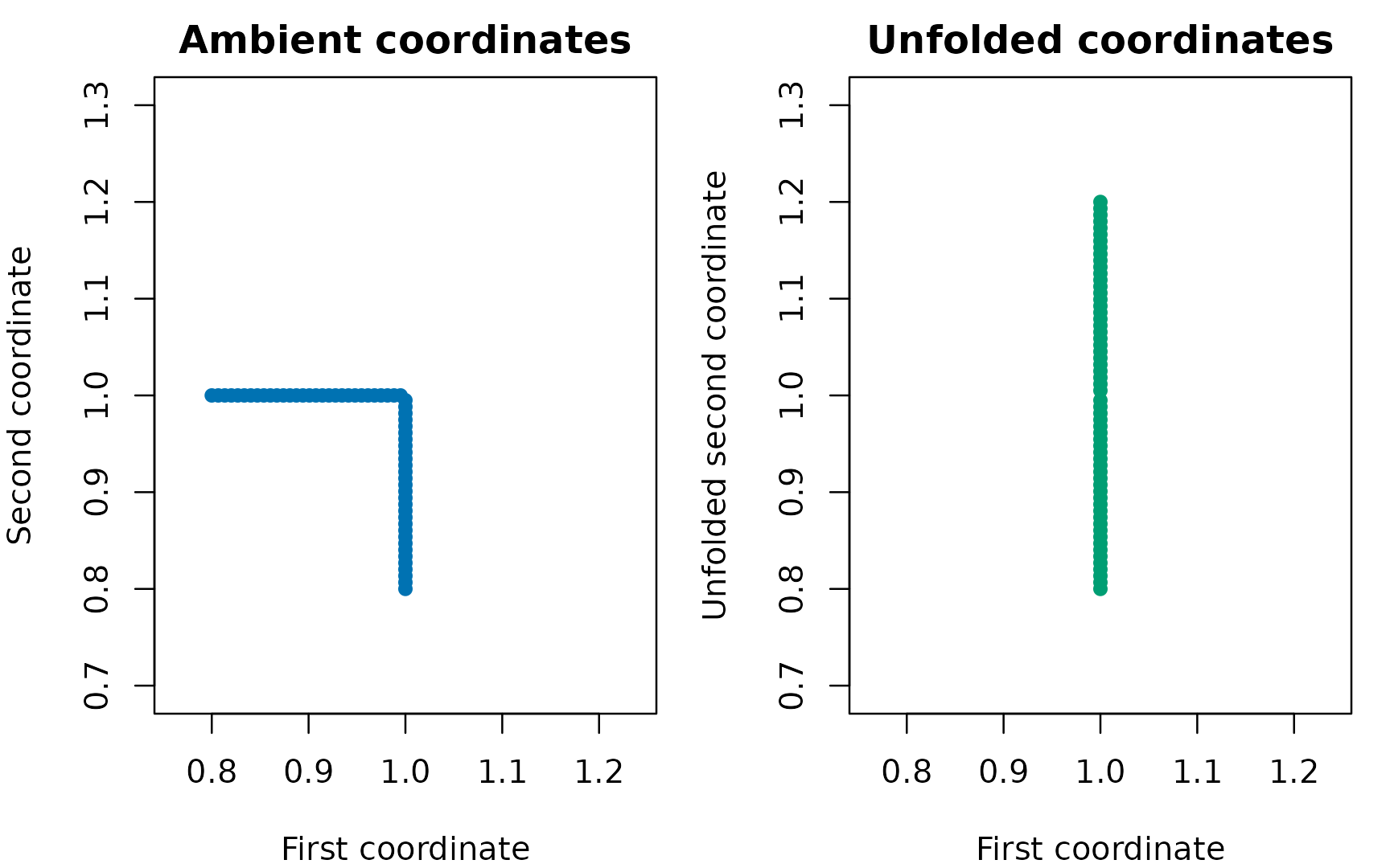

A straight latent coordinate appears bent in ambient coordinates. Unfolding rotates the adjacent face into the query face; both axes use the same physical scale.

par(old.par)
variance.one <- function(x) {
    values <- svd(scale(x, center=TRUE, scale=FALSE), nu=0, nv=0)$d^2
    values[1]/sum(values)
}
knitr::kable(data.frame(Chart=c("Ambient", "Unfolded"),
    `Variance retained by one PC (%)`=100*c(variance.one(seam),
        variance.one(flat$coordinates)), check.names=FALSE), digits=1)

Chart	Variance retained by one PC (%)
Ambient	80.4
Unfolded	100.0

Retaining more variance is a geometric result, not evidence of better outcome prediction. The examples below test prediction separately. Both folded and unfolded charts use the same intrinsic neighbors and weights. Unfolding can be rejected near corners, tied maxima or more than two faces; such cases are counted rather than silently forced into a chart.

Define examples before comparing methods

Each observation has six coordinates. The seam coordinate t and a broad coordinate u3 vary substantially. A narrow coordinate u4 has a much smaller range; the remaining two coordinates are nuisance features. The table gives the true log odds. The true probability is plogis(eta) and the observed response is a Bernoulli draw with that probability.

Example	True log odds, eta	Question
Seam	-1 + 2 t/0.2	Does a chart retain variation across the bend?
High variance	-1 + 2 (u3-0.3)/0.2	Can PCA capture a signal aligned with broad variation?
Low variance	-1 + 2 (u4-0.12)/0.02	Does supervised PLS recover a narrow signal direction?
Constant	-1	Does adaptation to binary noise hurt prediction?
Nonlinear	-1 + 2.5 ((t/0.2)^2 - 1/3)	How do local linear charts handle a symmetric nonlinear signal?

The narrow coordinate varies from 0.10 to 0.14. Its contribution to the log odds is deliberately as large as that of the broad coordinate in the high-variance example. This is a stress test for variance-based dimension reduction, not a claim about the frequency of such signals in real datasets. Predictor features are not standardized before constructing directions: doing so would change the geometry and would remove part of the contrast we intend to study. Component scores are scaled inside the local logistic fit.

scenarios <- c("Seam", "High variance", "Low variance", "Constant", "Nonlinear")
make.example <- function(seed, scenario, n=360L) {
    set.seed(seed)
    t <- runif(n, -.2, .2)
    X <- cbind(ifelse(t < 0, 1, 1-t), ifelse(t < 0, 1+t, 1),
               runif(n, .1, .5), runif(n, .10, .14),
               runif(n, .02, .06), runif(n, .02, .06))
    eta <- switch(scenario,
        "Seam"=-1+2*t/.2,
        "High variance"=-1+2*(X[,3]-.3)/.2,
        "Low variance"=-1+2*(X[,4]-.12)/.02,
        "Constant"=rep(-1,n),
        "Nonlinear"=-1+2.5*((t/.2)^2-1/3))
    probability <- plogis(eta)
    list(X=X, y=rbinom(n,1,probability), probability=probability, t=t)
}

Fit on training observations; choose dimension on tuning observations

Each of five independent repetitions per example has 180 training, 60 tuning and 120 test observations. The observations are independent in this simulation. For repeated specimens or matched sets, splitting must respect those groups instead.

We compare ambient PCA, unfolded PCA and unfolded PLS. All use 60 training neighbors, Gaussian weights, a fixed slope ridge penalty of 1, and half-success/ half-failure intercept pseudo-counts. Support size and ridge penalty are held fixed to make the chart comparison interpretable; they are not claimed optimal.

We report both a fixed one-dimensional chart and a chart dimension chosen from 1, 2 and 3 by the lowest tuning Brier loss. Ties choose the first (smaller) dimension. Tuning predictions use training observations only. Final test predictions use the same training fits; the tuning observations are not added to the training set. Test outcomes and true probabilities never select the model.

methods <- c("Ambient PCA", "Unfolded PCA", "Unfolded PLS")
fit.chart <- function(X, y, query, method, dimension, degree=1L) {
    fit.local.likelihood(X, y, X.eval=query, likelihood.family="bernoulli",
        chart.geometry="linf.simplex", unfold.faces=method != "Ambient PCA",
        coordinate.method=if (method == "Unfolded PLS") "local.pls" else "local.pca",
        support.size=60L, chart.dim=dimension, degree=degree,
        kernel="gaussian", lambda.ridge=1, intercept.mass=.5,
        max.iter=70L, tol=1e-7, fallback="degree0")
}
train <- 1:180
tune <- 181:240
test <- 241:360

Here is a complete fit for the low-variance example. Replacing "Unfolded PLS" with "Unfolded PCA" changes the directions while retaining the same geometry and likelihood settings.

dat <- make.example(271301, "Low variance")
fit <- fit.chart(dat$X[train,], dat$y[train], dat$X[test,],
                 "Unfolded PLS", dimension=1L)
head(fit$fitted.values)
fit$diagnostics$status.counts

The following loop executes the comparison. A local constant uses the same neighbors and weights but no chart directions. A global constant uses the smoothed overall training proportion. Both are useful controls, particularly when the true probability is constant.

rows <- list()
illustrations <- list()
append.result <- function(scenario, repetition, method, mode, dimension,
                          prediction, truth, response, fallbacks, tuning.fallbacks=NA_integer_) {
    stopifnot(all(is.finite(prediction)), all(prediction > 0 & prediction < 1))
    data.frame(scenario=scenario, repetition=repetition, method=method,
        mode=mode, dimension=dimension,
        probability.mse=mean((prediction-truth)^2),
        brier=mean((prediction-response)^2),
        log.loss=-mean(response*log(prediction)+(1-response)*log1p(-prediction)),
        fallbacks=fallbacks, tuning.fallbacks=tuning.fallbacks)
}
for (s in seq_along(scenarios)) for (repetition in 1:5) {
    scenario <- scenarios[s]
    dat <- make.example(271000+100*s+repetition, scenario)
    example.predictions <- list()
    for (method in methods) {
        fits <- lapply(1:3, function(d) fit.chart(dat$X[train,], dat$y[train],
            dat$X[c(tune,test),], method, d))
        tuning.loss <- vapply(fits, function(f)
            mean((f$fitted.values[1:60]-dat$y[tune])^2), numeric(1))
        best <- which.min(tuning.loss)
        for (mode in c("One dimension", "Tuned dimension")) {
            d <- if (mode == "One dimension") 1L else best
            chosen <- fits[[d]]
            prediction <- chosen$fitted.values[61:180]
            rows[[length(rows)+1L]] <- append.result(scenario, repetition, method,
                mode, d, prediction, dat$probability[test], dat$y[test],
                sum(chosen$diagnostics$per.eval$fallback[61:180]),
                sum(chosen$diagnostics$per.eval$fallback[1:60]))
            if (repetition == 1L) example.predictions[[paste(method,mode)]] <- prediction
        }
    }
    local <- fit.chart(dat$X[train,], dat$y[train], dat$X[test,],
                       "Ambient PCA", dimension=1L, degree=0L)
    constants <- list("Local constant"=local$fitted.values,
        "Global constant"=rep((sum(dat$y[train])+.5)/(length(train)+1), length(test)))
    for (method in names(constants)) {
        rows[[length(rows)+1L]] <- append.result(scenario, repetition, method,
            "Constant", 0L, constants[[method]], dat$probability[test], dat$y[test], 0L)
        if (repetition == 1L) example.predictions[[method]] <- constants[[method]]
    }
    if (repetition == 1L) illustrations[[scenario]] <- list(data=dat,
        predictions=example.predictions)
}
results <- do.call(rbind, rows)
stopifnot(nrow(results) == 200L)

Measure estimation and prediction separately

Probability mean squared error (MSE) compares the predicted probability with the known true probability. It directly measures estimation accuracy here. Brier loss compares the prediction with the binary response; it includes irreducible Bernoulli variation. Lower values are better for both. Test log loss is also retained in results for inspection. Neither a low MSE nor a converged optimizer alone establishes uncertainty calibration.

The table shows the mean across five repetitions. The figures show every repetition as well as the mean, so an apparently favorable average cannot hide a reversal. Five repetitions make a compact teaching example, not a powered simulation study or a universal ranking of methods.

summary.table <- aggregate(cbind(probability.mse,brier) ~ scenario+method+mode,
                           results, mean)
summary.table <- summary.table[order(match(summary.table$scenario, scenarios),
    match(summary.table$mode,c("One dimension","Tuned dimension","Constant")),
    match(summary.table$method,c(methods,"Local constant","Global constant"))),]
knitr::kable(summary.table, digits=4, row.names=FALSE,
    col.names=c("Example","Method","Chart","Probability MSE","Brier loss"))

Example	Method	Chart	Probability MSE	Brier loss
Seam	Ambient PCA	One dimension	0.0094	0.1753
Seam	Unfolded PCA	One dimension	0.0082	0.1727
Seam	Unfolded PLS	One dimension	0.0054	0.1677
Seam	Ambient PCA	Tuned dimension	0.0064	0.1677
Seam	Unfolded PCA	Tuned dimension	0.0067	0.1679
Seam	Unfolded PLS	Tuned dimension	0.0059	0.1678
Seam	Local constant	Constant	0.0084	0.1738
Seam	Global constant	Constant	0.0460	0.2171
High variance	Ambient PCA	One dimension	0.0076	0.1832
High variance	Unfolded PCA	One dimension	0.0092	0.1848
High variance	Unfolded PLS	One dimension	0.0054	0.1808
High variance	Ambient PCA	Tuned dimension	0.0062	0.1820
High variance	Unfolded PCA	Tuned dimension	0.0066	0.1817
High variance	Unfolded PLS	Tuned dimension	0.0074	0.1826
High variance	Local constant	Constant	0.0095	0.1848
High variance	Global constant	Constant	0.0465	0.2265
Low variance	Ambient PCA	One dimension	0.0473	0.2179
Low variance	Unfolded PCA	One dimension	0.0472	0.2178
Low variance	Unfolded PLS	One dimension	0.0473	0.2173
Low variance	Ambient PCA	Tuned dimension	0.0456	0.2132
Low variance	Unfolded PCA	Tuned dimension	0.0442	0.2107
Low variance	Unfolded PLS	Tuned dimension	0.0162	0.1929
Low variance	Local constant	Constant	0.0472	0.2180
Low variance	Global constant	Constant	0.0461	0.2165
Constant	Ambient PCA	One dimension	0.0025	0.1896
Constant	Unfolded PCA	One dimension	0.0029	0.1889
Constant	Unfolded PLS	One dimension	0.0037	0.1901
Constant	Ambient PCA	Tuned dimension	0.0034	0.1919
Constant	Unfolded PCA	Tuned dimension	0.0041	0.1916
Constant	Unfolded PLS	Tuned dimension	0.0041	0.1897
Constant	Local constant	Constant	0.0028	0.1899
Constant	Global constant	Constant	0.0005	0.1891
Nonlinear	Ambient PCA	One dimension	0.0180	0.2051
Nonlinear	Unfolded PCA	One dimension	0.0173	0.2047
Nonlinear	Unfolded PLS	One dimension	0.0099	0.1967
Nonlinear	Ambient PCA	Tuned dimension	0.0110	0.1924
Nonlinear	Unfolded PCA	Tuned dimension	0.0129	0.1928
Nonlinear	Unfolded PLS	Tuned dimension	0.0101	0.1965
Nonlinear	Local constant	Constant	0.0165	0.2036
Nonlinear	Global constant	Constant	0.0255	0.2095

colors <- c("Ambient PCA"="#0072B2", "Unfolded PCA"="#009E73",
    "Unfolded PLS"="#D55E00", "Local constant"="#666666", "Global constant"="#AA4499")
labels <- c("PCA", "Unfolded\nPCA", "Unfolded\nPLS", "Local\nconstant", "Global\nconstant")
old.par <- par(mfrow=c(5,2), mar=c(3.2,4,2,1), oma=c(0,0,1,0), cex=.8)
for (scenario in scenarios) for (mode in c("One dimension","Tuned dimension")) {
    tab <- results[results$scenario==scenario & results$mode %in% c(mode,"Constant"),]
    order.methods <- names(colors)
    plot(NA, xlim=c(.7,5.3), ylim=c(0, max(tab$probability.mse)*1.08+1e-6),
         xaxt="n", xlab="", ylab="Probability MSE", main=paste(scenario,mode,sep=" — "))
    axis(1, at=1:5, labels=labels, cex.axis=.8)
    for (j in 1:5) {
        values <- tab$probability.mse[tab$method==order.methods[j]]
        points(j+seq(-.12,.12,length.out=5), values, pch=16, cex=.7,
               col=adjustcolor(colors[j],alpha.f=.6))
        points(j, mean(values), pch=18, cex=1.3, col=colors[j])
    }
}

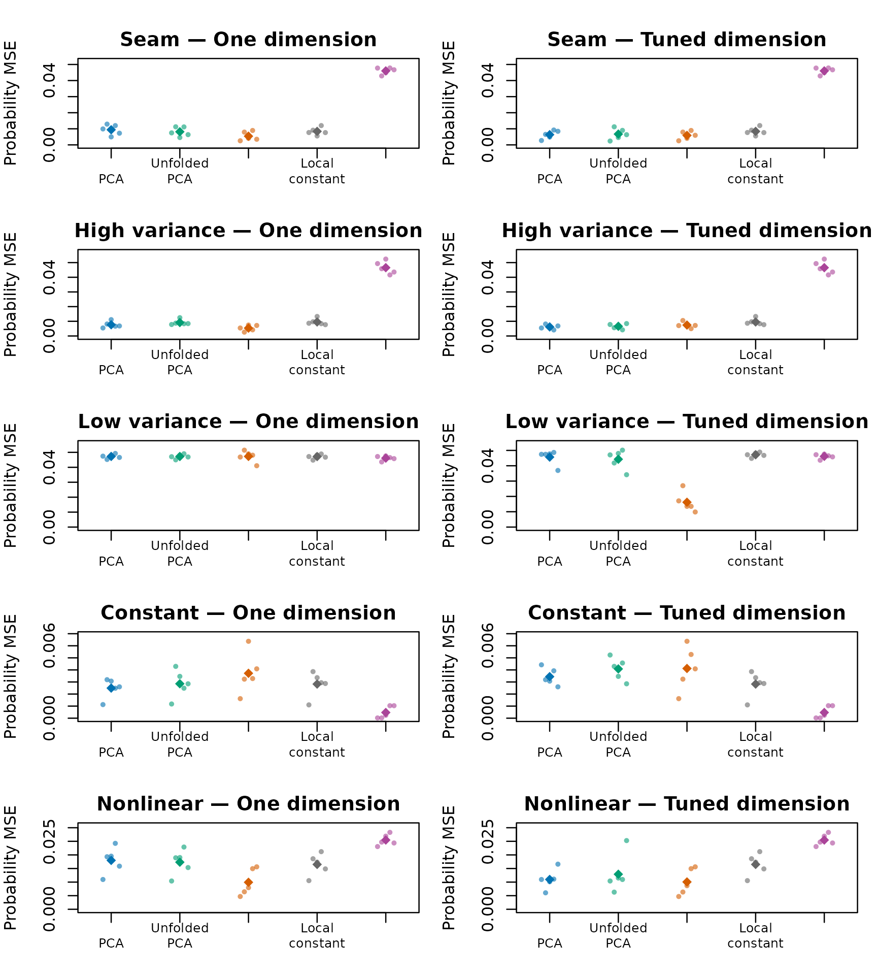
Held-out probability error for all five repetitions. Small points are independent repetitions; diamonds are their means. Each panel uses its own labelled vertical scale. Lower is better. The constant baselines are identical in the two columns.

par(old.par)

Inspect the first repetition, without choosing favorable seeds

The following plot compares predicted and true probabilities on the independent test observations from the first predeclared repetition of each example. Each point is one test observation. The diagonal is exact probability recovery, not a fitted regression line. Constant-probability observations share the same horizontal coordinate; vertical spread there shows adaptation to noise.

old.par <- par(mfrow=c(5,2), mar=c(3,3.3,2,1), cex=.8)
for (scenario in scenarios) for (method in c("Unfolded PCA","Unfolded PLS")) {
    item <- illustrations[[scenario]]
    prediction <- item$predictions[[paste(method,"One dimension")]]
    plot(item$data$probability[test], prediction, xlim=c(0,1), ylim=c(0,1),
         xlab="True probability", ylab="Predicted probability", pch=16, cex=.65,
         col=adjustcolor(colors[method],alpha.f=.55), main=paste(scenario,method,sep=" — "))
    abline(0,1,lty=2,col="grey35")
}

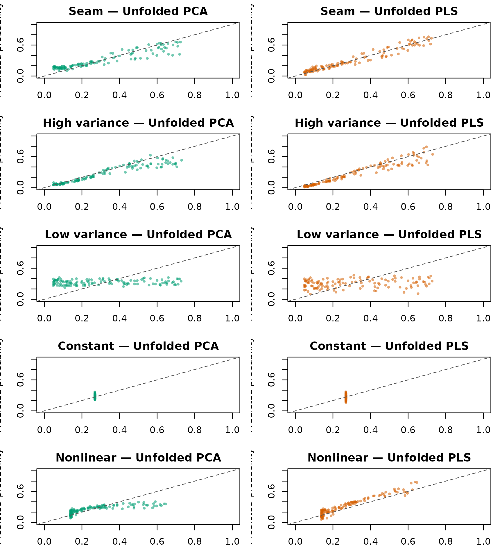
Predicted versus known true probabilities for first-repetition test observations. Columns compare unfolded PCA and PLS, each with one dimension. Points near the diagonal recover the true probabilities; all panels share the same axes.

par(old.par)

View the estimated probability functions

These slices use the first repetition’s training observations. The signal coordinate varies over its generating range while nuisance coordinates are held at the centers of their ranges. They show the fitted conditional function at defined locations, not averages of the scatterplots above. The black curve is the known truth. All methods use one-dimensional charts; they are not retuned on the displayed slices.

slices <- list()
old.par <- par(mfrow=c(3,2), mar=c(4,4,2,1), cex=.85)
for (scenario in scenarios) {
    grid <- seq(-1,1,length.out=60)
    t <- if (scenario %in% c("Seam","Nonlinear","Constant")) .2*grid else rep(.08,60)
    X.slice <- cbind(ifelse(t < 0,1,1-t), ifelse(t < 0,1+t,1), .3,.12,.04,.04)
    if (scenario=="High variance") X.slice[,3] <- .3+.2*grid
    if (scenario=="Low variance") X.slice[,4] <- .12+.02*grid
    eta <- if (scenario=="Constant") rep(-1,60) else if (scenario=="Nonlinear")
        -1+2.5*(grid^2-1/3) else -1+2*grid
    truth <- plogis(eta)
    dat <- illustrations[[scenario]]$data
    prediction <- vapply(methods, function(method)
        fit.chart(dat$X[train,],dat$y[train],X.slice,method,1L)$fitted.values,
        numeric(60))
    axis.value <- if (scenario=="High variance") X.slice[,3] else if (scenario=="Low variance")
        X.slice[,4] else t
    axis.label <- if (scenario=="High variance") "Broad coordinate u3" else if (scenario=="Low variance")
        "Narrow coordinate u4" else "Seam coordinate t"
    plot(axis.value,truth,type="l",lwd=2,col="black",ylim=c(0,1),
         xlab=axis.label,ylab="Probability",main=scenario)
    for (j in seq_along(methods)) lines(axis.value,prediction[,j],col=colors[j],lwd=1.5,lty=j)
    slices[[scenario]] <- list(X=X.slice,truth=truth,prediction=prediction)
}
plot.new()
legend("center",c("Truth",methods),col=c("black",colors[methods]),
       lty=c(1,1,2,3),lwd=c(2,1.5,1.5,1.5),bty="n",cex=.9)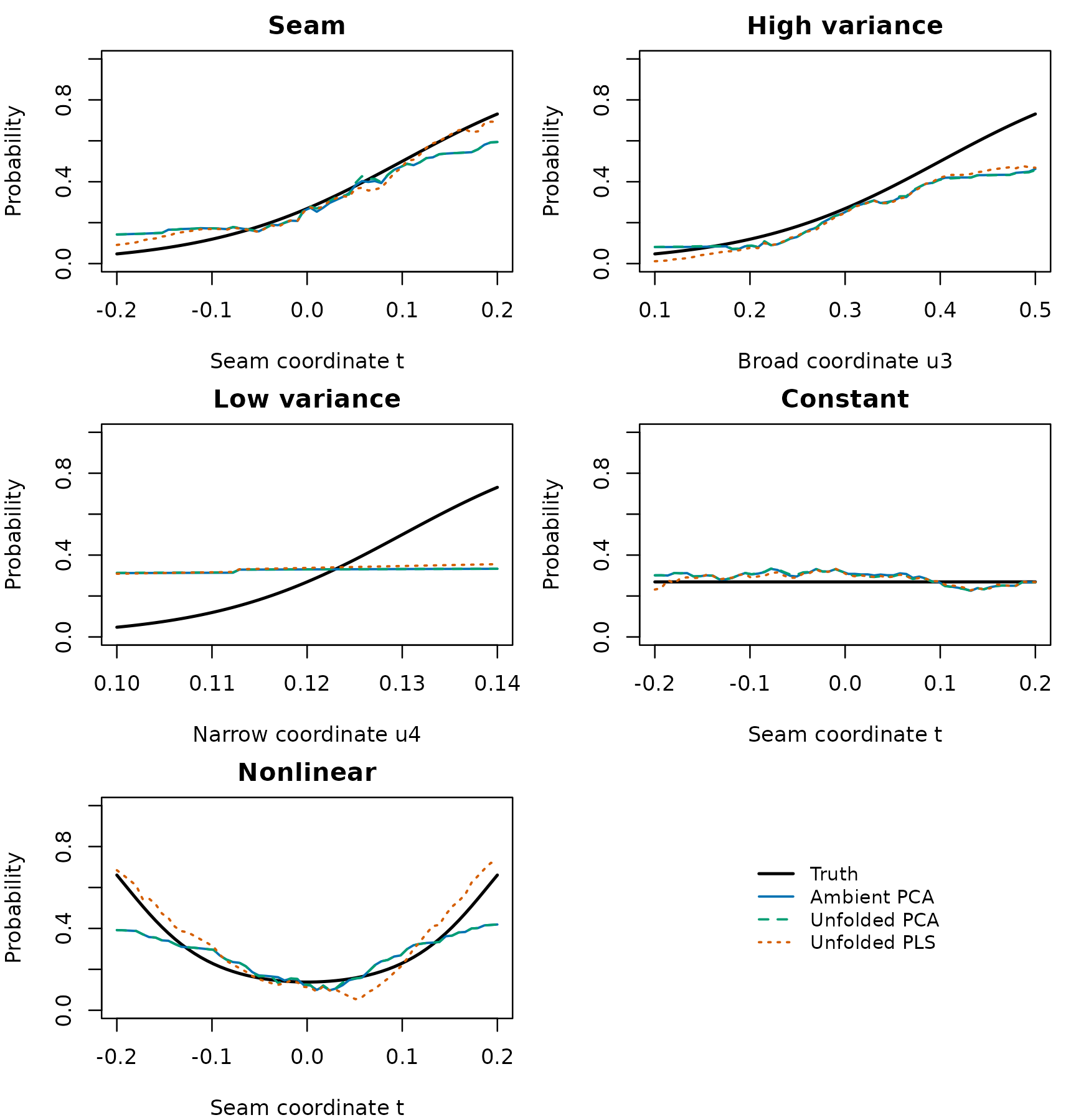

Conditional probability slices through the same first-repetition training fits. Nuisance coordinates are fixed at their generating centers. Black is the known truth; colored curves use one-dimensional charts. All probability axes run from zero to one.

par(old.par)

Check selected dimensions and fallbacks

tuned <- results[results$mode=="Tuned dimension",]
selection <- as.data.frame(xtabs(~scenario+method+dimension, tuned))
selection <- selection[selection$Freq>0,]
knitr::kable(selection, row.names=FALSE,
    col.names=c("Example","Method","Selected dimension","Repetitions"))

Example	Method	Selected dimension	Repetitions
Constant	Ambient PCA	1	3
High variance	Ambient PCA	1	3
Low variance	Ambient PCA	1	2
Nonlinear	Ambient PCA	1	1
Constant	Unfolded PCA	1	3
High variance	Unfolded PCA	1	2
Low variance	Unfolded PCA	1	1
Nonlinear	Unfolded PCA	1	1
Seam	Unfolded PCA	1	1
Constant	Unfolded PLS	1	4
High variance	Unfolded PLS	1	2
Nonlinear	Unfolded PLS	1	3
Seam	Unfolded PLS	1	4
Constant	Ambient PCA	2	1
High variance	Ambient PCA	2	2
Nonlinear	Ambient PCA	2	2
Seam	Ambient PCA	2	4
High variance	Unfolded PCA	2	2
Nonlinear	Unfolded PCA	2	2
Seam	Unfolded PCA	2	3
Constant	Unfolded PLS	2	1
High variance	Unfolded PLS	2	1
Nonlinear	Unfolded PLS	2	2
Seam	Unfolded PLS	2	1
Constant	Ambient PCA	3	1
Low variance	Ambient PCA	3	3
Nonlinear	Ambient PCA	3	2
Seam	Ambient PCA	3	1
Constant	Unfolded PCA	3	2
High variance	Unfolded PCA	3	1
Low variance	Unfolded PCA	3	4
Nonlinear	Unfolded PCA	3	2
Seam	Unfolded PCA	3	1
High variance	Unfolded PLS	3	2
Low variance	Unfolded PLS	3	5

knitr::kable(aggregate(cbind(fallbacks,tuning.fallbacks) ~ scenario+method+mode,
                      results, sum), row.names=FALSE,
    col.names=c("Example","Method","Chart","Test fallbacks","Tuning fallbacks"))

Example	Method	Chart	Test fallbacks	Tuning fallbacks
Constant	Ambient PCA	One dimension	0	0
High variance	Ambient PCA	One dimension	0	0
Low variance	Ambient PCA	One dimension	0	0
Nonlinear	Ambient PCA	One dimension	0	0
Seam	Ambient PCA	One dimension	0	0
Constant	Unfolded PCA	One dimension	0	0
High variance	Unfolded PCA	One dimension	0	0
Low variance	Unfolded PCA	One dimension	0	0
Nonlinear	Unfolded PCA	One dimension	0	0
Seam	Unfolded PCA	One dimension	0	0
Constant	Unfolded PLS	One dimension	0	0
High variance	Unfolded PLS	One dimension	0	0
Low variance	Unfolded PLS	One dimension	0	0
Nonlinear	Unfolded PLS	One dimension	0	0
Seam	Unfolded PLS	One dimension	0	0
Constant	Ambient PCA	Tuned dimension	0	0
High variance	Ambient PCA	Tuned dimension	0	0
Low variance	Ambient PCA	Tuned dimension	0	0
Nonlinear	Ambient PCA	Tuned dimension	0	0
Seam	Ambient PCA	Tuned dimension	0	0
Constant	Unfolded PCA	Tuned dimension	0	0
High variance	Unfolded PCA	Tuned dimension	0	0
Low variance	Unfolded PCA	Tuned dimension	0	0
Nonlinear	Unfolded PCA	Tuned dimension	0	0
Seam	Unfolded PCA	Tuned dimension	0	0
Constant	Unfolded PLS	Tuned dimension	0	0
High variance	Unfolded PLS	Tuned dimension	0	0
Low variance	Unfolded PLS	Tuned dimension	0	0
Nonlinear	Unfolded PLS	Tuned dimension	0	0
Seam	Unfolded PLS	Tuned dimension	0	0

A fallback is a failed chart certificate or failed optimizer replaced by the smoothed local proportion. Such predictions remain in the performance scores. They are not discarded to improve apparent performance. The table counts only reported rank-one or selected fits; its two modes reuse some fits and must not be added together as independent failures. results also retains each selected dimension and each test log loss.

Reading the comparison

The low-variance example shows why response-informed directions are not enough by themselves. With one dimension, unfolded PCA and PLS have mean probability MSEs of 0.0472 and 0.0473, respectively. After selecting dimension on the tuning observations, these become 0.0442 and 0.0162. Weighted PLS uses covariance and is still affected by predictor scale, binary noise and the number of retained directions. Its narrow-signal advantage here appears after dimension selection, not from its first direction alone.

The constant example favors the global constant in known-probability MSE. In the high-variance example, dimension-tuned PCA has a smaller mean probability MSE than dimension-tuned PLS. Dimension tuning itself sometimes worsens test performance relative to the one-dimensional fit: 60 tuning observations give a noisy selection criterion. These comparisons explain why the vignette shows baselines, fixed and selected dimensions, and every repetition.

The seam example distinguishes correcting a geometric fold from learning a response direction. The high-variance example is favorable to PCA’s criterion; the low-variance example deliberately puts important response information in a direction PCA may discard. Increasing the chart dimension gives PCA a chance to recover that information, with additional estimation variability. PLS can help at low dimension, but its supervised directions must be learned exclusively from training data.

The constant example is an essential control: there is no informative direction to recover. The nonlinear example asks whether local neighborhoods make a nonlinear function adequately linear; the local PLS covariance can be weak near symmetry points even when the response depends strongly on position. No method is assumed to win these comparisons. Differences among individual repetitions, not just averages, matter.

For a scientific analysis, expand the simulation to realistic sample sizes, class balance, dependence, missingness and geometry. Tune support size and regularization inside training data, assess probability calibration on an outer hold-out sample, and examine performance near corners or low-support regions. For case-control sampling, recovering conditional probability in the selected sample does not identify population prevalence without sampling information.

Reproduce and adapt

All results and figures are computed by this vignette. No cohort data, saved outcome fits or Python reference predictions are read. The 25 seeds and all settings are fixed in the code. The workload is serial; it can be rendered with single-threaded BLAS/OpenMP to avoid competing with other analyses. See ?fit.local.likelihood and ?unfold.simplex.chart for controls and diagnostics.

#> [1] '0.2.0'
#> [1] '0.4.1'