Synthetic datasets for geometric smoothing

For the complete task and function catalog, see Finding your way around geosmooth.

geosmooth represents a synthetic dataset as four serializable components: geometry, sampling, truth, and response. synthetic.spec() combines those components without drawing data. materialize.synthetic() performs all random work under an explicit seed and RNG policy and returns a validated synthetic_dataset.

library(geosmooth)

circle.spec <- synthetic.spec(
  geometry = dgraphs::synthetic.circle(radius = 1, ambient.dim = 2),
  sampling = dgraphs::synthetic.sampling.grid.interval(
    0, 2 * pi, endpoints = "exclude.lower"),
  truth = synthetic.truth.polynomial(c(b0 = 0)),
  response = synthetic.response.gaussian(sd = 0.05)
)
circle.data <- materialize.synthetic(circle.spec, n = 80, seed = 2026)
circle.data
#> <synthetic_dataset> adhoc__specd155e302ac4d6d54d5298f321d3b01cbba0f539a0eaca5e892e69502f3fce186__n80__seed2026__rngnamed.stream.v1
#>   n=80  intrinsic=1  ambient=2  truth=population

The circle has one latent coordinate (angle) and two observed coordinates (the embedding). The constant truth is intentional: this recipe isolates response noise around zero, rather than testing recovery of a varying signal.

old.par <- par(mfrow = c(1, 2), mar = c(4, 4, 2, 1))
plot(circle.data, view = "geometry", col = "#0072B2", asp = 1,
     main = "Observed geometry")
plot(circle.data, view = "response", col = "grey40", xlab = "Angle (radians)",
     main = "Response and truth")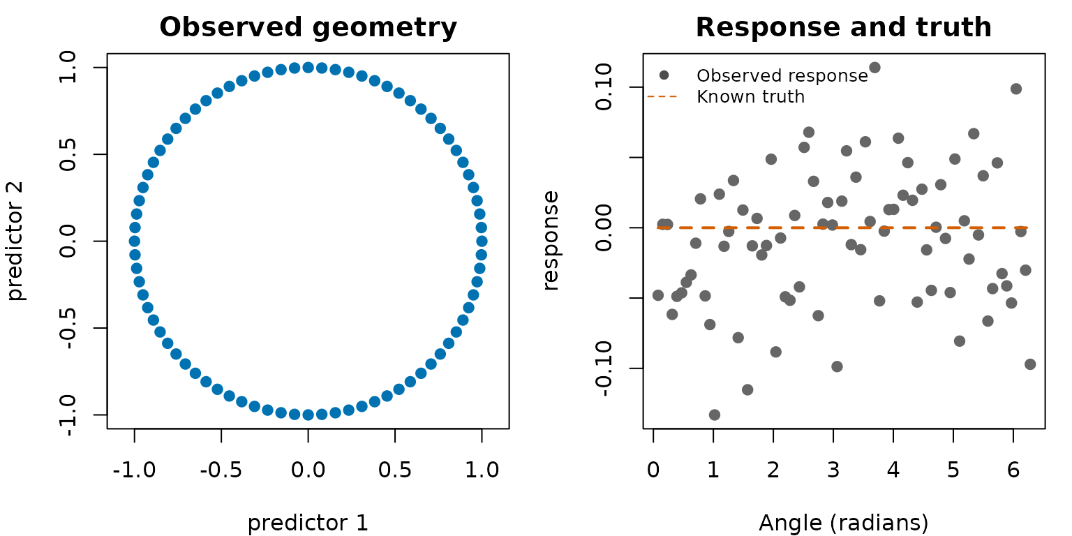

Left: the circle in its two observed coordinates. Right: responses versus latent angle, with the constant zero truth shown by a dashed line. These views describe the same 80 observations.

par(old.par)

Quadforms use separate intrinsic and ambient dimensions. A flat geometry has no quadratic forms; a paraboloid or saddle supplies one or more symmetric forms.

surface.spec <- synthetic.spec(
  geometry = dgraphs::synthetic.quadform(
    intrinsic.dim = 2,
    ambient.dim = 5,
    forms = list(diag(c(1, -1))),
    frame = "random.orthonormal"
  ),
  sampling = dgraphs::synthetic.sampling.uniform.box(-1, 1),
  truth = synthetic.truth.polynomial(c(b0 = 0, b1 = 1, b22 = -0.5)),
  response = synthetic.response.gaussian(sd = 0.1)
)
surface.data <- materialize.synthetic(surface.spec, n = 100, seed = 17)
dim(surface.data$latent)
#> [1] 100   2
dim(surface.data$predictors)
#> [1] 100   5
head(as.data.frame(surface.data))
#>                                                                                                      dataset.id
#> 1 adhoc__spec90adf9b19cf8db3041878a96a32d5b64aefa1f3bcd1b727a58bb377520b71d2f__n100__seed17__rngnamed.stream.v1
#>   recipe.id registry.tag   n intrinsic.dim ambient.dim truth.scope
#> 1      <NA>         <NA> 100             2           5  population
#>        rng.policy
#> 1 named.stream.v1
#>                                                           checksum
#> 1 45387e61a4a08f29cf4686a7d874d01ccb15e23994eb9eacbd2573d7087abbc5

The surface has two latent coordinates and five observed coordinates. The random orthonormal frame embeds the surface in five dimensions. Viewing two coordinates is a projection: points that appear close may be separated in coordinates omitted from the display.

plot(surface.data, view = "geometry", color = "truth", main = "Projected surface")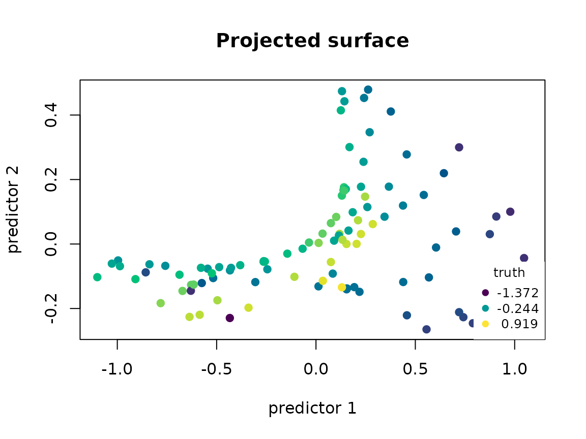

Two-coordinate projection of a surface embedded in five dimensions. Point colors indicate the known, nonconstant conditional mean; the key uses its actual numerical range.

This second recipe has a varying polynomial truth. A smoother receives the observed predictors and noisy response, not the latent coordinates or truth:

surface.fit <- fit.lps(surface.data$predictors, surface.data$response,
  foldid = rep(1:5, length.out = surface.data$n),
  support.grid = c(20L, 30L), degree.grid = 1L,
  kernel.grid = "gaussian", coordinate.method = "local.pca", chart.dim = 2L)
surface.fit$selected
#>   support.size degree   kernel bandwidth.multiplier candidate.id chart.dim
#> 2           30      1 gaussian                    1            2         2
#>   cv.rmse.observed
#> 2        0.1237177
head(data.frame(response = surface.data$response, fitted = fitted(surface.fit),
                truth = surface.data$truth))
#>     response     fitted      truth
#> 1 -1.0535767 -1.0190866 -0.9362011
#> 2  0.3064608  0.3704115  0.3825321
#> 3 -0.6452932 -0.6436731 -0.5908854
#> 4  0.8054648  0.8094692  0.7589337
#> 5 -1.2332430 -1.4065217 -1.3718367
#> 6 -0.3173372 -0.2974997 -0.2596817

The fitted values are on the observed rows. Truth is available for this synthetic demonstration only; selecting settings and reporting their CV score does not supply an independent test of prediction accuracy. The first-fit guide explains that distinction.

Maintained benchmark recipes are discoverable through synthetic.registry.ids(). G1–G7 remain compatibility identifiers; the S01–S16 shape identifiers and V1–V3 sampling/noise variants preserve the shared SSRHE regression suite. For example, S01.V1 means two separated narrow equal signal peaks with uniform sampling and Gaussian response noise. G1 is an ambient polynomial example; G2 is a polynomial on a flat embedded geometry. Ordinary datasets bind their full specification hash into dataset.id.

ids <- c("G1", "G2", "S01.V1")
do.call(rbind, lapply(ids, function(id) {
  spec <- synthetic.registry.spec(id)
  data.frame(id, geometry = spec$geometry.spec$family,
             truth = spec$truth.spec$parameters$estimand)
}))
#>       id geometry
#> 1     G1 quadform
#> 2     G2 quadform
#> 3 S01.V1 quadform
#>                                                               truth
#> 1                                       Polynomial conditional mean
#> 2                                       Polynomial conditional mean
#> 3 Gaussian-mixture signal normalized by its realized design maximum
registered <- synthetic.registry.spec("S01.V1")
registered.data <- materialize.synthetic(
  registered, n = 160,
  seed = synthetic.registry.seed("S01.V1", replicate = 1),
  rng.policy = "legacy"
)
synthetic.dataset.checksum(registered.data)
#> [1] "e1d4d84ca14d8446a8f559cdb0f694595091a87a3c6d5e8b8e26cd3d590d5cc8"

Use rng.policy = "named.stream.v1" for new work. The "legacy" policy exists for frozen scientific parity and pins historical RNG behavior. Predictor noise, response noise, and finite-design truth normalization are distinct contracts; they should not be substituted for one another.