Finding your way around geosmooth

geosmooth estimates a response or probability mass on coordinate data and graphs. Start with the task you want to perform, then choose a method. You do not need to learn the operator constructors or synthetic-data helpers to fit your first model.

Choose a starting point

Your task	Start here	What to know before choosing
Regress a response on coordinates	fit.lps()	Local polynomial smoothing; selects neighborhood size, degree, and kernel by cross-validation.
Average predictions from overlapping local models	fit.malps()	Model-averaged local polynomial smoothing; supports coordinate and graph-geodesic neighborhoods.
Couple local polynomial predictions across overlaps	fit.ps.lps()	Prediction-synchronized local polynomial smoothing; experimental R reference implementation.
Fit a locally adaptive trend with a sparse difference penalty	fit.lpl.tf()	Local polynomial lifting trend filtering; requires optional package genlasso.
Add synchronization to a lifting trend filter	fit.slpl.tf()	Synchronized local polynomial lifting trend filtering; adds a second, quadratic penalty.
Smooth a response already attached to graph vertices	fit.metric.graph.lowpass() or fit.graph.trend.filtering()	Choose spectral low-pass smoothing or a graph-difference penalty. Edge-weight meanings differ; see below.
Penalize local second derivatives on a point cloud	fit.ssrhe.hessian.regression()	Hessian-energy regression, following semi-supervised regression using Hessian energy (SSRHE); use lambda.selection = "cv" or "gcv" to select penalties.
Use an absolute-value Hessian penalty	fit.ssrhe.hessian.l1.regression()	Different regularization from quadratic Hessian energy; has its own solver and tuning controls.
Interpolate graph values while fixing a region boundary	perform.harmonic.smoothing()	Iterative harmonic relaxation; harmonic.smoother() also records extrema and topology diagnostics.
Estimate probability mass over a fixed support	fit.density()	Takes nonnegative counts or masses; returns mass over the rows of X.
Estimate where one subject visits that support	fit.subject.od()	Takes visit indices, including repeats; handles occupation-density fitting and optional visit-level validation.
Build reproducible synthetic examples	synthetic.spec() then materialize.synthetic()	Combine geometry, sampling, truth, and response noise.

These choices describe different estimators, not a ranking of predictive performance. Parallel-transport trend filtering and transported graph Hessians have their own experimental section.

A first regression fit

Use X with one observation per row and a response y of matching length. A local chart is a coordinate system fitted near an observation, often using principal component analysis (PCA). Start in the supplied coordinates before adding local charts or changing numerical controls.

library(geosmooth)
set.seed(1)
X <- matrix(seq(0, 1, length.out = 60), ncol = 1)
truth <- sin(2 * pi * X[, 1])
y <- truth + rnorm(nrow(X), sd = 0.08)
fit <- fit.lps(
  X, y, foldid = rep(1:5, length.out = nrow(X)),
  support.grid = c(8L, 12L, 16L), degree.grid = 0:1,
  kernel.grid = "gaussian"
)
fit$selected
#>   support.size degree   kernel bandwidth.multiplier candidate.id chart.dim
#> 4            8      1 gaussian                    1            4         1
#>   cv.rmse.observed
#> 4       0.07990112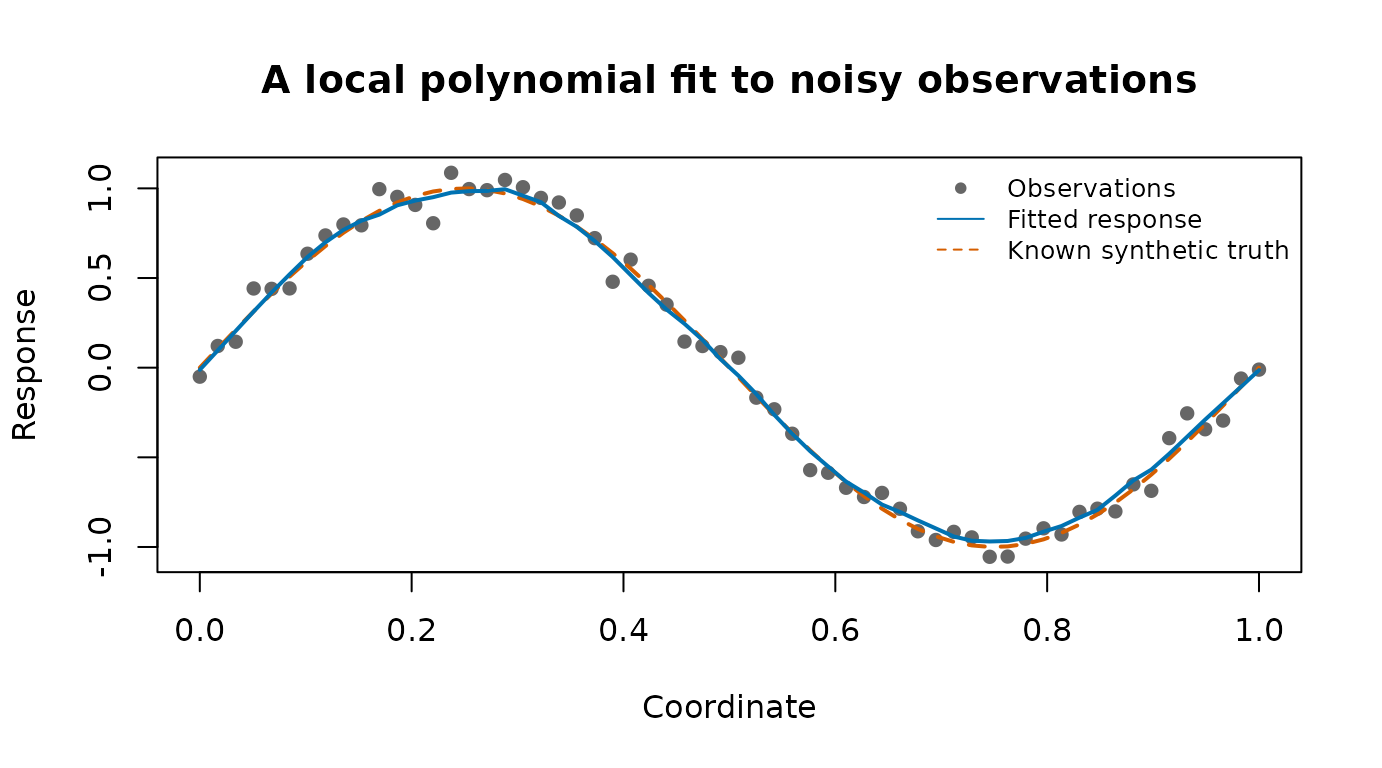

The points are noisy observations. The solid blue line is the selected fit; the dashed orange line is known only because these data are synthetic.

Here CV selected 8-point neighborhoods, degree 1, and the Gaussian kernel, with a tuning RMSE of 0.0799 response units. A larger support averages more nearby responses; the polynomial degree determines the local shape. The selected CV score was used for tuning, so it is not an independent measure of performance. This small illustration shows how to read a fit; it does not rank estimators.

head(fitted(fit))
#> [1] -0.01193899  0.09633293  0.20478722  0.31316459  0.41899355  0.52015223
new.X <- matrix(seq(0.1, 0.9, length.out = 5), ncol = 1)
predict(fit, newdata = new.X)
#> [1]  0.593224184  0.978163565  0.003195166 -0.910822694 -0.559835093

Cross-validation (CV) holds out responses to choose tuning parameters. A support is the neighborhood used for a local fit; a grid lists candidate values. The local support size and polynomial degree jointly determine whether a local fit has enough observations. For grouped observations, use lps.grouped.foldid() to keep each group in one fold. Use lps.nested.cv() when you need an outer assessment of the whole tuning procedure.

Prediction and reusable fits

Fitted object	How to get predictions	Scope
Local polynomial smoother	predict(fit) or predict(fit, newdata = Xnew)	Existing evaluation points or new coordinate rows.
Model-averaged local polynomial smoother	predict(fit) or predict(fit, newdata = Xnew)	New coordinates are supported for coordinate-distance fits; graph-geodesic fits currently reject new targets.
Either lifting trend filter	predict(fit)	Training points only; newdata must be NULL.
Prediction-synchronized, chart-kernel, local-likelihood, graph low-pass, graph trend-filtering, Hessian, or parallel-transport fit	fitted(fit)	No registered predict() method for these classes in this version. Chart-kernel and local-likelihood fits can receive X.eval when fitting.
Density or occupation-density result	fit$rho	Probability mass on the evaluation support.
Tracked harmonic result (harmonic.smoother())	fitted(fit)	Values on the original graph vertices.
Basic harmonic result (perform.harmonic.smoothing())	fit$harmonic_predictions	An unclassed list; retains the basic function’s original contract.

Use summary(fit) for selected settings and stored diagnostics. The summary explicitly says when convergence information is unavailable. fitted(fit) preserves the vector or matrix stored by each regression fit. residuals(fit) preserves missing-label masks and requires an aligned response: a fit evaluated at other coordinates has no training residuals. These are response-scale residuals, including for binomial fits; they are not Pearson or deviance residuals. See help("model-values", package = "geosmooth") and help("model-summary", package = "geosmooth") for the contracts. Probability mass remains fit$rho; it is a different quantity.

A refit changes the response while reusing geometry or an operator. It does not automatically rerun the original model-selection procedure. Each refit method documents whether penalties remain fixed or can be selected again. An operator describes the differences or derivatives being penalized; it is not itself a fitted response. A spectral basis stores graph eigenvectors so many responses can be smoothed without recomputing them.

Refit and extract smoother matrices

Use refit(fit, y = new.y, ...) for all six reusable model families. R chooses the method from the fitted object’s class. The controls in the last column belong to that method; they are not shared by every model.

Fitted model	Accepted response	Geometry reused and tuning behavior
MALPS	Vector; omitted or NULL reuses the stored response	Supports and averaging weights stay fixed. Optional weights affect local coefficient estimation; robust residual weights are recomputed.
Lifting trend filter	Vector required	Reuses the residual operator and stored penalty, or accepts a fixed lambda.
Synchronized lifting trend filter	Vector required	Reuses both operators and stored penalties, or accepts fixed lambda1 and lambda2.
Metric graph low-pass	Vector or matrix required	Reuses the spectral basis and smoothing parameter; per.column.gcv = TRUE selects a parameter for each response column.
Quadratic Hessian-energy regression	Vector or matrix; omitted or NULL reuses the stored response	Reuses the operator and fixed penalties; accepts lambda1, lambda2, weights, and ridge. CV/GCV fits dispatch here and retain their selected penalties by default.
Hessian L1 regression	One response; omitted or NULL reuses the stored response	Reuses the derivative operator; accepts lambda.grid, fixed or CV lambda.selection, and solver controls.

For repeated metric graph low-pass or quadratic Hessian refits, keep using the original fitted object. Their returned refit summaries cannot themselves be refitted. The other four families return reusable fitted objects.

Use smoother.matrix(fit, ...) for LPS and MALPS. LPS accepts check.tol and returns a map from training responses to evaluation predictions under its fixed-configuration restrictions. MALPS accepts max.n and allow.robust and returns a training-point matrix conditional on stored supports and weights. For robust MALPS, allow.robust = TRUE freezes the final robust weights; it does not capture their response-dependent changes.

malps.fit <- fit.malps(
  X, y, degree = 1L, support.type = "knn", support.size = 12L
)
new.y <- cos(2 * pi * X[, 1])
malps.refit <- refit(malps.fit, y = new.y)
S <- smoother.matrix(malps.fit)
max(abs(as.vector(S %*% new.y) - predict(malps.refit)))
#> [1] 4.440892e-16

The former six refit.*() entry points and two *.smoother.matrix() entry points are no longer exported. Replace fitted.model = with object = and y.new = with y = in old refit calls. Other method-specific arguments and return classes are unchanged. help("refit", package = "geosmooth") and help("smoother.matrix", package = "geosmooth") link to each method’s full argument list; former help names remain available.

Function catalog

Each row in the geosmooth catalog gives one exported name and its purpose. In an R session, open the corresponding help with, for example, help("fit.lps", package = "geosmooth"). The final two sections explicitly list related functions owned by dgraphs; they are not geosmooth exports, and their detailed help lives in dgraphs.

Shared model operations

Function	Purpose
refit()	Refit a supported model with a new response using stored geometry and method-specific tuning controls.
smoother.matrix()	Extract the conditional linear map for a supported LPS or MALPS fit.

Local regression and prediction synchronization

Function	Purpose
fit.lps()	Fit and tune local polynomial regression, including supported Gaussian and binary response modes.
fit.malps()	Fit and optionally tune a model-averaged collection of local polynomial models.
fit.ps.lps()	Fit experimental local polynomial models whose predictions are synchronized on overlaps.
fit.chart.kernel()	Fit a chart-kernel field, with optional reference-measure quadrature weights.
fit.local.likelihood()	Fit local density or Bernoulli likelihood models; returns a fitted field.

Model assessment and uncertainty

Function	Purpose
lps.grouped.foldid()	Assign whole groups of observations to validation folds.
lps.nested.cv()	Assess a tuned local polynomial smoother using outer and inner validation folds.
lps.backend.diagnostics()	Inspect the computational backend, chart dimensions, and selected controls.
lps.pointwise.band()	Calculate pointwise uncertainty for a supported fixed-configuration Gaussian fit.
malps.gcv()	Calculate generalized cross-validation and optional leave-one-out diagnostics for a stored model-averaged fit.
bootstrap.malps()	Measure refit variability by bootstrap case weights while holding the selected geometry fixed.

Generalized cross-validation (GCV) uses a smoother’s effective degrees of freedom to estimate prediction error without explicitly fitting every leave-one-out model. It is not interchangeable with every form of CV.

The two uncertainty workflows have different assumptions. LPS uncertainty requires a Gaussian fit, the R backend, the documented orthogonal polynomial basis, a single candidate configuration, and a fixed chart dimension. Its pointwise band also requires evaluation at the training points. MALPS matrix and bootstrap diagnostics condition on the selected supports and weights; they do not repeat model selection. Neither workflow provides simultaneous coverage or automatic uncertainty for a full data-selected pipeline.

Lifting trend filters

Function	Purpose
lpl.tf.operator()	Build a local polynomial residual operator.
fit.lpl.tf()	Fit a trend filter with an absolute-value penalty on those residuals.
slpl.tf.operator()	Build the residual operator together with an overlap synchronization operator.
fit.slpl.tf()	Fit the residual penalty plus quadratic synchronization.

Both fitters accept a prebuilt operator or can construct one. For a single fit, start with the fitter. Build operators explicitly when comparing responses, studying neighborhoods, or reusing expensive geometry. Both fitters currently require genlasso; their supported prediction domain is the training set.

Graph spectral smoothing and graph trend filtering

Function	Purpose
fit.metric.graph.lowpass()	Select a graph-spectral smoothing parameter by GCV and fit a response.
metric.graph.lowpass.operator()	Convert metric edge lengths to conductances and construct a graph Laplacian.
metric.graph.lowpass.basis()	Construct and retain graph eigenvectors for repeated smoothing.
apply.metric.graph.lowpass.path()	Apply a supplied basis over a parameter grid; retain the candidate fits.
metric.graph.heat.eta.grid()	Choose heat-time candidates using spectral information.
metric.graph.heat.extend.lower()	Propose a smaller heat time for an external search, subject to resolution safeguards.
graph.trend.filtering.operator()	Construct graph differences or experimental path divided differences.
fit.graph.trend.filtering()	Fit an absolute-value graph-difference penalty; requires genlasso.

Graph construction and shortest paths are supplied by dgraphs. A graph’s adjacency list contains 1-based vertex indices; a parallel weight list gives the corresponding edge values. Check their meaning for the chosen method: metric low-pass smoothing interprets them as lengths and converts them to conductances. Recursive graph trend filtering uses conductance-like weights, whereas its path divided-difference option uses lengths. Conductance measures connection strength; it is not the same quantity as distance.

Heat time (eta) controls the amount of spectral smoothing. A truncated basis can fail to resolve small positive heat times; use the returned spectral diagnostics when constructing or extending a path yourself.

From a constructed graph to a fitted response

This example uses the tested development dependency described in the README; the compatible dgraphs release must be on CRAN before geosmooth 0.2.0 is submitted. The 20 locations form an undirected chain because the construction radius joins only adjacent sites. Vertex i, coordinate row i, and response entry i refer to the same observation. Retain your identifiers in a separate table and join by those identifiers before fitting; a smoother cannot detect a shuffled response.

# Each row, vertex, and response refers to the same location.
locations <- matrix(seq(0, 1, length.out = 20), ncol = 1,
                    dimnames = list(sprintf("site-%02d", 1:20), "position"))
response <- sin(2 * pi * locations[, 1])
graph <- dgraphs::create.rknn.graph(locations, radius = .06,
                                    graph.detail = "minimal")
# dgraphs' new dgraph representation has public accessors. The second branch
# supports the pinned transitional dependency used by this development release.
if (inherits(graph, "dgraph")) {
  adjacency <- dgraphs::graph.adjacency(graph)
  edge.lengths <- dgraphs::graph.lengths(graph)
} else {
  adjacency <- graph$adj_list
  edge.lengths <- graph$weight_list
}
graph.fit <- fit.metric.graph.lowpass(
  adjacency, edge.lengths, response,
  n.eigenpairs = nrow(locations), eigen.solver = "dense",
  conductance.rule = "inverse.length.power", conductance.alpha = 1,
  conductance.epsilon = 1e-8, eta.grid = c(.001, .01, .1, 1)
)
head(data.frame(site = rownames(locations), response,
                fitted = fitted(graph.fit)))
#>            site  response      fitted
#> site-01 site-01 0.0000000 0.006105107
#> site-02 site-02 0.3246995 0.324089090
#> site-03 site-03 0.6142127 0.612949746
#> site-04 site-04 0.8371665 0.835444574
#> site-05 site-05 0.9694003 0.967406378
#> site-06 site-06 0.9965845 0.994534692
graph.fit$gcv[c("eta.optimal", "gcv.optimal", "effective.df")]
#> $eta.optimal
#> [1] 0.001
#> 
#> $gcv.optimal
#> [1] 0.0002323874
#> 
#> $effective.df
#> [1] 19.2978
# Reuse the fitted object's spectral basis, with the selected smoothing fixed.
second.fit <- refit(graph.fit, y = cos(2 * pi * locations[, 1]))
head(fitted(second.fit))
#> [1]  0.99896194  0.94388145  0.78751744  0.54582318  0.24498057 -0.08240949

With conductance.alpha = 1, a length of 2 becomes a conductance of 1 / (2 + 1e-8), approximately 0.5. Longer edges therefore connect responses less strongly. This choice changes the smoothing operator; it is not just a change of labels. The example retains all eigenvectors, so no spectral truncation is involved. For large graphs, use the spectral diagnostics described in help("metric.graph.lowpass.basis") when retaining fewer eigenvectors. The second response reuses those eigenvectors and the selected heat time. The printed GCV score is a tuning criterion, not held-out predictive error.

Input context	Meaning	Consequence
Coordinate neighborhoods	Distances in the supplied coordinate units	Rescaling coordinates changes supports.
Graph-geodesic neighborhoods	Sums of edge lengths along paths	Unreachable vertices have infinite distance; support rules must handle connectivity.
Metric low-pass smoothing	Positive lengths transformed to conductances	Reciprocal edges and matching lengths are required; zero lengths are rejected.
Recursive graph differences	Conductance-like weights	Greater weight penalizes differences more strongly.
Path divided differences	Edge lengths	The operator uses metric spacing, not conductance.

For example, metric.graph.lowpass.operator(list(2L, integer()), list(1, numeric())) is rejected because the edge has no reciprocal entry. Do not repair directed or zero-length input silently. Resolve its scientific meaning before choosing a supported undirected positive-length graph.

Hessian-energy regression

Function	Purpose
ssrhe.hessian.operator()	Estimate local derivative operators and Hessian-energy matrices from point-cloud neighborhoods.
fit.ssrhe.hessian.regression()	Fit quadratic Hessian-energy regression using fixed penalties, label CV, or GCV; optionally select supports.
fit.ssrhe.hessian.l1.regression()	Fit an absolute-value derivative penalty with fixed or CV-selected regularization.
ssrhe.support.grid()	Build candidate adaptive-radius support profiles for tuning.

The Hessian describes local second derivatives. A quadratic penalty spreads curvature reduction across the fitted field; an absolute-value penalty can set derivative components to zero. These are different estimators.

Label CV supports semi-supervised use: some vertices may lack an observed response. GCV currently requires one fully observed response vector and strictly positive observation weights. Exact GCV traces and randomized trace estimates have different computational costs and reproducibility properties. For the absolute-value fitter, solver = "admm" selects the implemented alternating direction method of multipliers; the genlasso solver requires that optional package.

To select quadratic Hessian penalties, use the same fitter with an explicit selection mode. Mode-specific settings belong in cv.control or gcv.control. Scalar penalties and candidate grids cannot be combined.

hessian.fit <- fit.ssrhe.hessian.regression(
  X, y, k = 12L, tangent.dim = 1L,
  lambda.selection = "cv", lambda1.grid = c(0.01, 0.1),
  cv.control = list(foldid = rep(1:5, length.out = nrow(X)))
)
hessian.fit$lambda
#> $lambda1
#> [1] 0.01
#> 
#> $lambda2
#> [1] 0
#> 
#> $ridge
#> [1] 0

The former .cv() and .gcv() fitter names have been retired. Their old help names still lead to the unified fitter’s migration instructions. Existing fixed calls with lambda1 and optional lambda2 continue to work.

Harmonic interpolation

Function	Purpose
perform.harmonic.smoothing()	Relax interior values while holding the region boundary fixed; return convergence diagnostics.
harmonic.smoother()	Run relaxation while recording extrema, prediction history, and topology stability.
get.region.boundary()	Find region vertices with a neighbor outside the region.

Use print(), summary(), and plot() on the tracked harmonic_smoother object. The two smoothing functions currently differ in boundary-free behavior so they should not be treated as aliases. In the current native implementation, boundary vertices are defined by a neighbor outside the region; a degree-one vertex inside a whole-graph region is not automatically fixed. The basic function returns unchanged input with status = "no_boundary" when no boundary exists; the tracked function still runs relaxation. Both require small value changes and a small harmonic residual for numerical convergence. Extrema stability is a separate diagnostic: stability_detected records whether a window was found, and stable_iteration is NA otherwise. On an alternating path, recording every second iteration can appear stable while the values continue to oscillate. Check converged and max_residual; a stability detection does not establish optimal smoothing.

Probability mass and subject occupation

Function	Purpose
fit.density()	Fit empirical or graph-random-walk mass estimates from nonnegative weights on a support.
normalize.density()	Convert a numeric field or supported fitted object to probability mass, with normalization diagnostics.
fit.subject.od()	Convert repeated visit indices into counts and fit a subject-occupation distribution.

support <- matrix(seq(0, 1, length.out = 6), ncol = 1)
occupation <- fit.subject.od(
  support, subject.index = c(1L, 3L, 3L, 6L), method = "empirical"
)
occupation$rho
#> [1] 0.25 0.00 0.50 0.00 0.00 0.25
sum(occupation$rho)
#> [1] 1

Here the third support point receives twice as many visits as the first or sixth. rho is a probability mass vector over support points, summing to one; it is not automatically a continuous density per unit volume. normalize.density() is an explicit conversion step, not another regression fit. Inspect its clipping and normalization accounting when the source field contains negative values.

fit.subject.od() offers more methods than fit.density(): it can fit ordinary smoothers and normalize their output. Visit-level CV holds out visits and uses visit.foldid; ordinary regression CV holds out support rows and uses foldid (or the method-specific spelling). Keep these validation units distinct.

Experimental transport methods

Function	Purpose
pttf.geometry()	Build local tangent frames and their transport across a graph.
pttf.operator()	Construct parallel-transport trend-filtering differences from that geometry.
pttf.operator.filter.rows()	Select operator rows while maintaining provenance and related operator data.
fit.pttf.trend.filtering()	Fit a parallel-transport trend filter with an absolute-value or quadratic penalty.
transported.graph.hessian.operator()	Build a separate experimental graph Hessian diagnostic with several direction-matching rules.

Parallel transport aligns local tangent directions before comparing derivatives. These experimental interfaces expose geometry, operator, and solver diagnostics deliberately. The transported graph Hessian constructor is a separate diagnostic workflow; it does not fit a response and is not an interchangeable spelling of pttf.operator().

Synthetic datasets: specifications, responses, and reproducibility

Function	Purpose
synthetic.spec()	Combine geometry, sampling, truth, and response descriptors without drawing data.
materialize.synthetic()	Draw a dataset from a specification with an explicit seed and random-number policy.
materialize.synthetic.instance()	Reproduce a registered frozen instance and optionally validate its checksum.
synthetic.registry.ids()	List maintained recipe identifiers.
synthetic.registry.spec()	Look up a recipe specification; some recipe families allow parameter overrides.
synthetic.registry.seed()	Reproduce legacy SSRHE recipe seeds; this is not a seed generator for every registry family.
validate.synthetic.dataset()	Check the structure and consistency of a materialized dataset.
compare.synthetic.dataset()	Compare two datasets with explicit numerical tolerances.
synthetic.dataset.checksum()	Compute a content checksum for reproducibility checks.
synthetic.sampling.stratified()	Describe allocation between the supported synthetic strata.
synthetic.truth.named()	Select a named truth specification with optional parameters.
synthetic.truth.polynomial()	Specify polynomial truth in the chosen evaluation coordinates.
synthetic.truth.gaussian.mixture()	Specify Gaussian-mixture truth using centers, scales, and weights.
synthetic.truth.occupation.mixture()	Specify occupation-mixture truth with covariance and probability controls.
synthetic.truth.logit()	Specify a logit-based truth with prevalence and clipping controls.
synthetic.response.gaussian()	Specify Gaussian response noise with a supplied standard deviation.
synthetic.response.heteroskedastic.gaussian()	Specify Gaussian noise whose scale depends on truth.
synthetic.response.clustered.gaussian()	Specify within-cluster correlated Gaussian noise.
synthetic.response.laplace.outlier()	Specify Laplace noise and an outlier component.
synthetic.response.bernoulli()	Specify binary response draws and optional positive-count requirements.

The constructors create specifications; materialize.synthetic() performs random draws. Use print(), plot(), and as.data.frame() on a resulting synthetic_dataset. For complete examples, read vignette("synthetic-datasets", package = "geosmooth"). Use the named-stream random-number policy for new work; historical seed and algorithm controls preserve frozen examples and should not be changed casually.

Geometry constructors and helpers supplied by dgraphs

These names are available from dgraphs, and are no longer exported by geosmooth. Replace former geosmooth:: calls with dgraphs::. See, for example, help("synthetic.circle", package = "dgraphs").

Function	Purpose
dgraphs::synthetic.circle()	Describe a circle or circular arc and its embedding.
dgraphs::synthetic.helix()	Describe a helical curve.
dgraphs::synthetic.trefoil()	Describe a trefoil curve.
dgraphs::synthetic.torus.patch()	Describe a patch of a torus.
dgraphs::synthetic.sphere.cap()	Describe a spherical cap.
dgraphs::synthetic.quadform()	Describe a flat or quadratic geometry with intrinsic and ambient dimensions.
dgraphs::synthetic.simplex()	Describe a simplex with a given number of parts.
dgraphs::synthetic.stratified()	Combine strata and optional junctions.
dgraphs::synthetic.stratum.point()	Describe a point stratum.
dgraphs::synthetic.stratum.segment()	Describe a line-segment stratum.
dgraphs::synthetic.stratum.rectangle()	Describe a rectangular stratum.
dgraphs::synthetic.point.line.junction()	Describe a point-and-line junction geometry.
dgraphs::embed.synthetic.geometry()	Map latent coordinates to the ambient space.
dgraphs::edge.lengths.synthetic.geometry()	Evaluate geometry-aware lengths between latent endpoints.
dgraphs::quadform.gradient()	Evaluate the gradient of a quadratic geometry.
dgraphs::quadform.metric()	Evaluate its induced metric.

Sampling constructors supplied by dgraphs

Function	Purpose
dgraphs::synthetic.sampling.uniform.interval()	Describe uniform draws on an interval.
dgraphs::synthetic.sampling.uniform.box()	Describe uniform draws in a box.
dgraphs::synthetic.sampling.uniform.rectangle()	Describe uniform draws in a rectangle with its specified draw algorithm.
dgraphs::synthetic.sampling.uniform.disk()	Describe uniform draws in a disk.
dgraphs::synthetic.sampling.grid.interval()	Describe an interval grid with an endpoint convention.
dgraphs::synthetic.sampling.gapped.uniform()	Describe sampling across separated intervals.
dgraphs::synthetic.sampling.truncated.normal()	Describe bounded Gaussian draws.
dgraphs::synthetic.sampling.clustered()	Describe clustered observations around random centers.
dgraphs::synthetic.sampling.dirichlet.zeros()	Describe Dirichlet sampling with structural zeros.

Similar geometric domains do not imply identical random-number sequences: these descriptors also preserve ordering and algorithm choices.

Finding detailed help

Function links in this guide open the rendered online reference. When working without an internet connection, the same help is installed with the package: use help("fit.lps", package = "geosmooth"), replacing fit.lps with the function name. Start at help("geosmooth-package", package = "geosmooth") for clickable task links in installed help, or use browseVignettes("geosmooth") for the installed HTML guides.

The synthetic datasets guide develops reproducible geometry, sampling, truth, and response specifications in more detail.

help(package = "geosmooth")
help("geosmooth-package", package = "geosmooth")
help("fit.lps", package = "geosmooth")
help("predict.lps", package = "geosmooth")
vignette("function-guide", package = "geosmooth")
vignette("synthetic-datasets", package = "geosmooth")

The package’s help pages give exact arguments, defaults, return values, and examples. Use this guide to find the appropriate family, then read the chosen function’s help before configuring its advanced controls.

Advanced controls without a new fitter

Each main fitter’s installed help groups controls for a first fit, selection, geometry, numerical solving, and returned diagnostics. Begin with a small statistical grid; numerical tolerances do not replace statistical tuning.

Family	Fold and selection vocabulary	Meaning and main cost
LPS / MALPS	foldid, cv.folds, support/degree/kernel grids	Held-out response selection; candidate combinations multiply fitting work.
Quadratic Hessian	lambda.selection, cv.control, gcv.control	Label CV or GCV; exact trace calculation is more expensive than sampled traces.
Hessian L1	fold.id, nfolds, lambda.grid, admm.*	CV excludes unconverged solves; each candidate and fold needs a solve.
Graph low-pass	eta.grid, n.eigenpairs	GCV over heat times; a full spectral basis uses quadratic storage.

smoother.matrix() returns a dense evaluation-by-training matrix. Retained candidate fits and solver histories also consume memory. Request them for an actual diagnostic purpose. These differences are deliberate method contracts; matching argument names would not make the criteria equivalent.

The catalog covers all explicitly exported functions in geosmooth 0.2.0. Geometry and sampling functions are owned by dgraphs. Registered methods are accessed through familiar generics; use the installed package index for the complete method list rather than treating methods as additional fitters.