geosmooth provides geometric methods for nonparametric regression and density estimation on data represented as coordinate matrices or weighted graphs. It includes local polynomial smoothing, model-averaged local polynomial smoothing, local polynomial lifting trend filtering, synchronized local polynomial lifting trend filtering, graph low-pass filtering, and Hessian-energy regression.
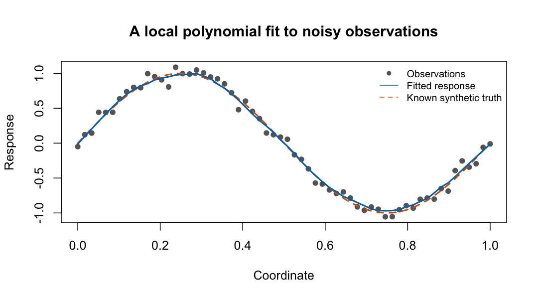
The points are observations, the solid line is a selected local polynomial fit, and the dashed line is known synthetic truth. The first-fit guide shows the code, selected settings, and how to interpret the tuning score.
For a task-based catalog of every exported function, prediction capabilities, and examples, read Finding your way around geosmooth. In an installed package, use vignette("function-guide", package = "geosmooth") or start with help("geosmooth-package", package = "geosmooth").
Browse the reference by task, functions A–Z, or synthetic datasets guide. See NEWS for migration details.
Installation
For the version currently on CRAN:
install.packages("geosmooth")
help("geosmooth-package", package = "geosmooth")
The development version (0.2.0) includes the guides below and requires a newer dgraphs than CRAN currently supplies. Its optional GRIP and edge-KK embeddings also require the current dot-delimited grip API. Install the tested dependency revisions explicitly; installing from changing main branches is not an equivalent dependency specification. A source installation needs an R compilation toolchain.
install.packages("pak")
pak::pkg_install(c(
  "pgajer/ivue@a952ab6816636a19f2038ba0709181608b71770d",
  "pgajer/dgraphs@e7cde950dd86a411f1d41e707392789d33f5617c",
  "pgajer/grip@07dc145c89ff31b399a7e4c0b8e1b86f391fc08b",
  "pgajer/geosmooth"
))
vignette("function-guide", package = "geosmooth")
Development CI uses those same dependency revisions. The separate CRAN dependency check workflow installs dependencies exclusively from CRAN and must pass before submission. A compatible dgraphs release is still a prerequisite for releasing geosmooth 0.2.0. The pinned dgraphs revision includes the R-devel synthetic RNG-state compatibility fix. The grip API used by the optional embeddings must also be available on CRAN before release. The development checks do not establish CRAN-only release readiness.
Quick Start
library(geosmooth)

set.seed(1)
x <- seq(0, 1, length.out = 60)
X <- cbind(x = x)
y <- sin(2 * pi * x) + rnorm(length(x), sd = 0.08)
foldid <- rep(1:5, length.out = length(y))

lps.fit <- fit.lps(
    X = X,
    y = y,
    foldid = foldid,
    support.grid = c(8L, 12L, 16L),
    degree.grid = 0:1,
    kernel.grid = "gaussian"
)

head(predict(lps.fit))
fit.lps() is the canonical local polynomial smoother (LPS) entry point. It selects support size, local polynomial degree, and kernel by cross-validation.
Method Map
Choose by the structure of your data and the penalty you need:
LPS: local polynomial smoother,
fit.lps(). Use this as the direct local-regression baseline. It predicts by fitting a local polynomial around each evaluation point.MALPS: model-averaged local polynomial smoother,
fit.malps(). Use this when you want many local polynomial fits around observed anchors and an averaged prediction surface.LPL-TF: local polynomial lifting trend filtering,
fit.lpl.tf()andlpl.tf.operator(). Use this when the local polynomial residual operator should be regularized by an L1 (absolute-value) trend-filtering penalty.SLPLiFT / S-LPL-TF: synchronized local polynomial lifting trend filtering,
fit.slpl.tf()andslpl.tf.operator(). Use this when you want LPL-TF plus a quadratic synchronization penalty across overlapping local predictions.Graph low-pass:
fit.metric.graph.lowpass()smooths a response on an undirected graph with positive edge lengths. The graph workflow explains vertex alignment, length-to-conductance conversion, and basis reuse.SSRHE: SSRHE-style Hessian-energy smoothing,
fit.ssrhe.hessian.regression()andfit.ssrhe.hessian.l1.regression(). Use this as a Hessian-energy comparator with fixed-k, supplied, or graph-derived adaptive-radius neighborhoods.
Basic Examples
MALPS
malps.fit <- fit.malps(
    X = X,
    y = y,
    degree = 1L,
    support.type = "knn",
    support.size = 12L,
    kernel = "tricube",
    support.selection = "fixed",
    coordinate.method = "coordinates"
)
LPL-TF and SLPLiFT Operators
lpl.op <- lpl.tf.operator(
    X = X,
    degree = 1L,
    support.type = "knn",
    support.size = 12L,
    kernel = "gaussian",
    coordinate.method = "coordinates"
)

slpl.op <- slpl.tf.operator(
    X = X,
    degree = 1L,
    support.type = "knn",
    support.size = 12L,
    kernel = "gaussian",
    coordinate.method = "coordinates"
)
Fitting LPL-TF and SLPLiFT currently uses the optional genlasso dependency.
if (requireNamespace("genlasso", quietly = TRUE)) {
    lpl.fit <- fit.lpl.tf(
        y = y,
        operator = lpl.op,
        lambda = 0.1,
        lambda.selection = "fixed"
    )

    slpl.fit <- fit.slpl.tf(
        y = y,
        operator = slpl.op,
        lambda1 = 0.1,
        lambda2 = 0.01,
        lambda.selection = "fixed"
    )
}
SSRHE Hessian-Energy Regression
grid <- expand.grid(x = seq(0, 1, length.out = 5),
                    y = seq(0, 1, length.out = 5))
X2 <- as.matrix(grid)
y2 <- sin(2 * pi * X2[, 1]) + 0.25 * X2[, 2]

ssrhe.fit <- fit.ssrhe.hessian.regression(
    X = X2,
    y = y2,
    k = 12L,
    tangent.dim = 2L,
    lambda1 = 0.05,
    return.local.diagnostics = FALSE
)

# Select penalties with the same fitter (use "gcv" for fully observed data).
ssrhe.cv <- fit.ssrhe.hessian.regression(
    X = X2,
    y = y2,
    k = 12L,
    tangent.dim = 2L,
    lambda.selection = "cv",
    lambda1.grid = c(0.01, 0.05, 0.2),
    cv.control = list(cv.folds = 5L)
)
The same runnable code is available in inst/examples/geosmooth_quickstart.R.
Graph Dependency Boundary
geosmooth owns smoother APIs and package-local coordinate/fixed-k paths. Graph construction and shortest-path operations are supplied by dgraphs.
That means:
- Coordinate LPS, coordinate MALPS, coordinate LPL-TF/SLPLiFT, fixed-k SSRHE, and supplied-neighborhood SSRHE are package-local
geosmoothpaths. - Graph-dependent paths, including graph-geodesic MALPS/LPL-TF/SLPLiFT supports and SSRHE adaptive-radius neighborhoods, use compatible
dgraphsgraph objects. -
geosmoothdoes not currently export graph construction functions such as rKNN graph builders.
Native support currently includes:
- C++ coordinate backend for LPS CV and prediction
- C++ shared local-PCA chart backend
- C++ SSRHE Hessian-energy operator backend