Plot Geodesic Statistics — plot.geodesic

Creates visualizations of geodesic statistics to help understand the relationship between radius and number of geodesics.

Usage

# S3 method for class 'geodesic_stats'
plot(
  x,
  plot.type = c("summary", "heatmap", "vertex", "all"),
  selected.vertices = NULL,
  max.vertices = 10,
  ...
)

Arguments

x: List. Output from compute.geodesic.stats().
plot.type: Character. Type of plot to generate: "summary" (default), "heatmap", "vertex", or "all".
selected.vertices: Integer vector. Specific vertices to highlight in "vertex" plots. If NULL, a random sample will be used.
max.vertices: Integer. Maximum number of vertices to show in vertex plot.
...: Additional arguments passed to summary

Value

Invisibly returns NULL.

Examples

stats <- list(
  radii = c(0.2, 0.4),
  geodesic_rays = matrix(c(2, 3, 3, 4), nrow = 2, byrow = TRUE),
  composite_geodesics = matrix(c(1, 1, 1, 2), nrow = 2, byrow = TRUE),
  grid_vertices = c(5L, 9L),
  summary = data.frame(
    radius = c(0.2, 0.4),
    avg_rays = c(2.5, 3.5),
    max_rays = c(3, 4),
    composite_ratio = c(0.4, 0.5),
    avg_overlap_median = c(0.35, 0.45)
  )
)
class(stats) <- c("geodesic_stats", "list")

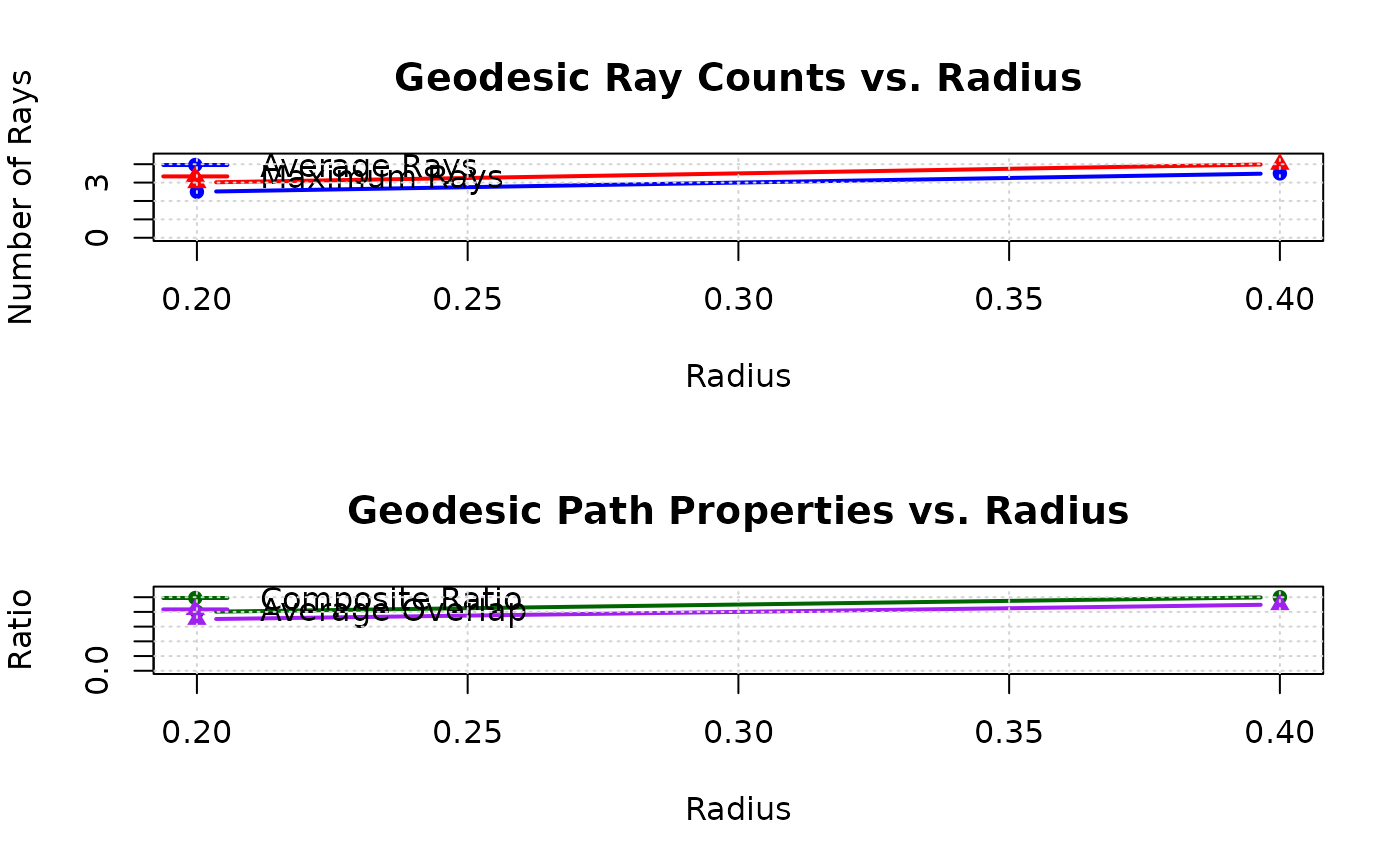
plot(stats, plot.type = "summary")

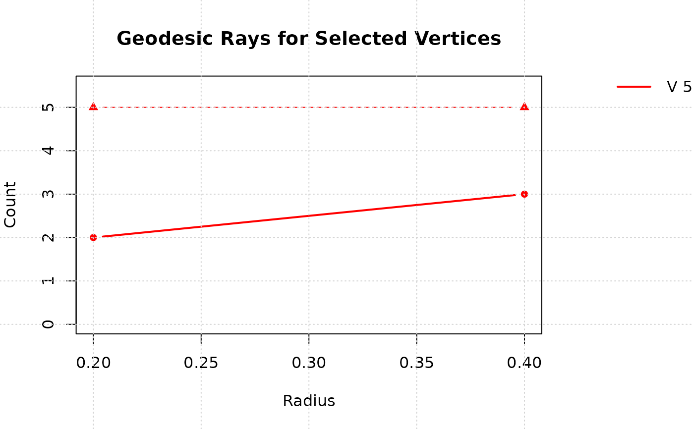
plot(stats, plot.type = "vertex", selected.vertices = 5)